In this project, I transformed images into user-defined shapes by way of a 3 x 3 homography matrix. By doing this, we can rectify images to change the perceived camera angle as well as stitch images together to create fluid panorama pictures.

I then implemented non-maximal suppression, feature matching, and RANSAC in order to fully automate the painstaking process of choosing feature points for generating the projective transformation homography.

A Beautiful View of the Bay from Lawrence Hall of Sciences

First, we capture an image with a preferably rectangular object. We must then collect 4 pairs of feature points in order to recover the homography matrix H.

3 x 3 Homography Matrix H

Here is an example of the feature points I selected:

Corners of the Sign Selected

Destination Locations of the Selected Points

We can use the corners of the object in the original image and then map them to a set of coordinates pertaining to a rectangular shape. For the best results, the rectangle should be about the same size as the original object.

Given our input image feature points (x, y) shown above on the left and our rectangular points (u, v) shown above on the right, we can construct the following equation in the form of Ah = b:

Matrix Representation of the Equation: Ah = b

We can then solve for the matrix h by solving the system of equations. We take our resulting h vector and transform it into the 3 x 3 matrix H with an arbitrary value of 1 in the bottom right corner. Then given a point in our original image:

p = [x, y, 1]^T

we can apply our matrix H to get from this point to the point warped into the coordinate space of our other set of feature points. Namely, the equation is:

Hp = p'

where p' = [wx', wy', w]^T

We can figure out the size of our output image by forward transforming our corners to see where they map to in our new coordinate space. Once we've calculated the size of our output image, we can simply take each coordinate of the output image and inverse warp it, that is run the point through the equation:

(H^-1)p' = p

This way, we can find the coordinate in the original image that we need to copy the color for for our point p'. We must also remember that p' will be in the form of:

p' = [wx', wy', w]^T

So we need to divide each index by w to get the homogeneous coordinates. A last note is that some points in the output image will not map to points in the original image prior to warping. If such a point p is encountered, we simple ignore it and leave the pixel in the output image black.

A few of my better results are displayed below:

Original

Rectified

Original

Rectified

Original

Rectified

As you can see, when we rectify the image we can make the image seem to be taken from a different angle. This is most drastically seen in the first pair of images where we shift the camera up and take an overhead view of the stone in the ground.

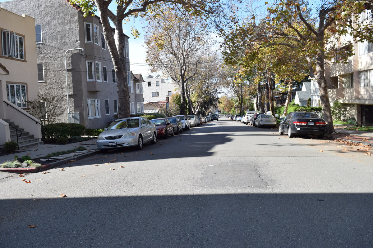
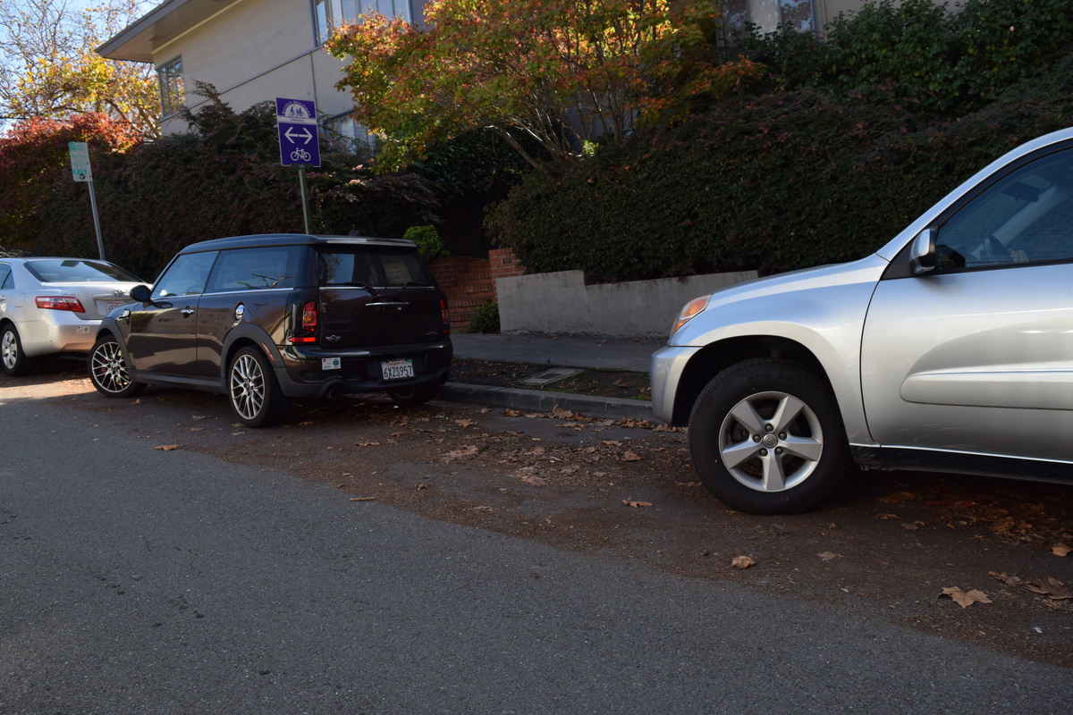
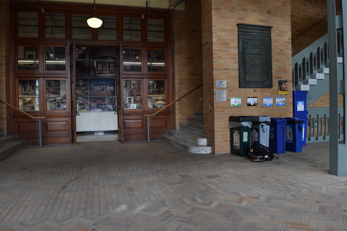
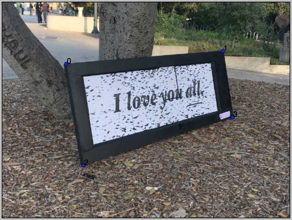
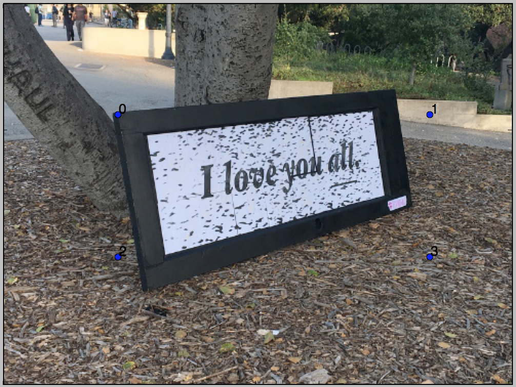
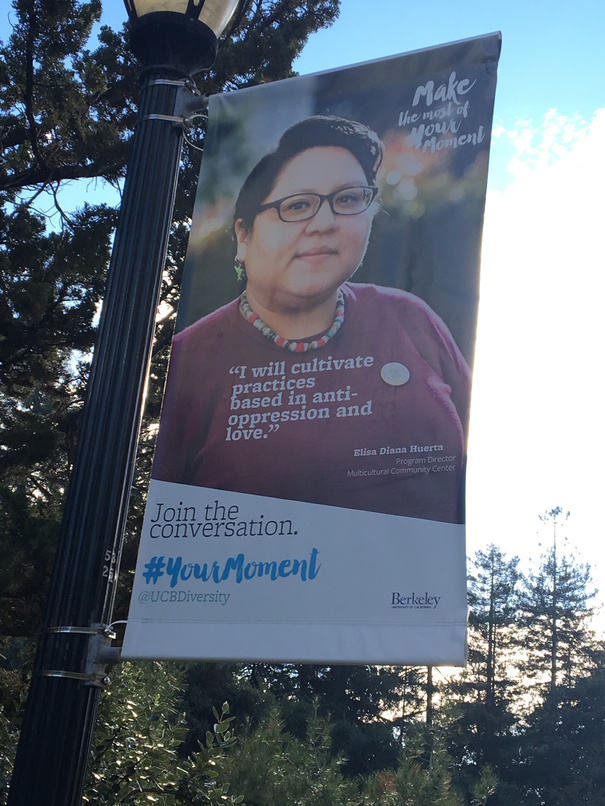
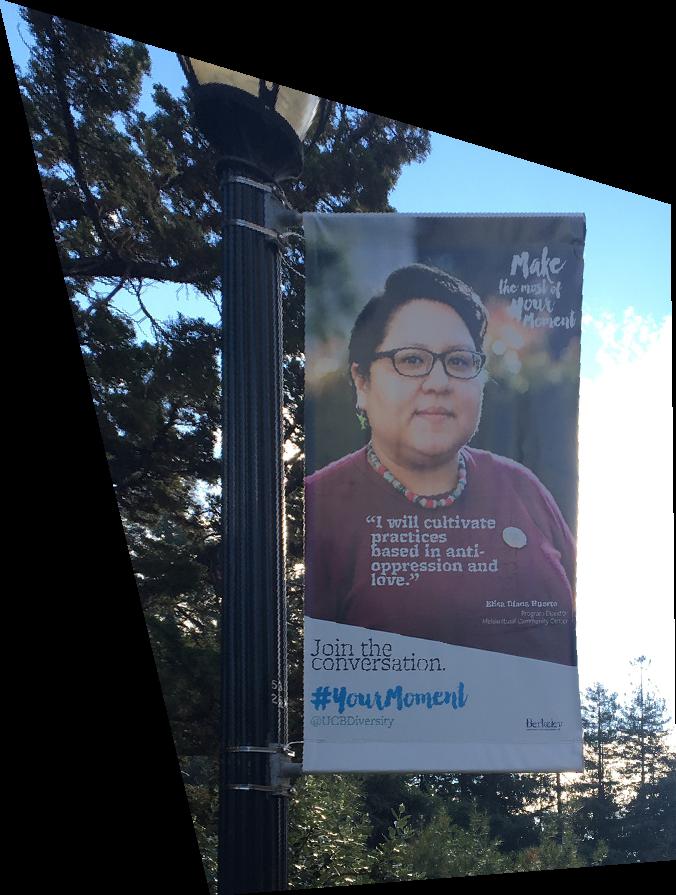
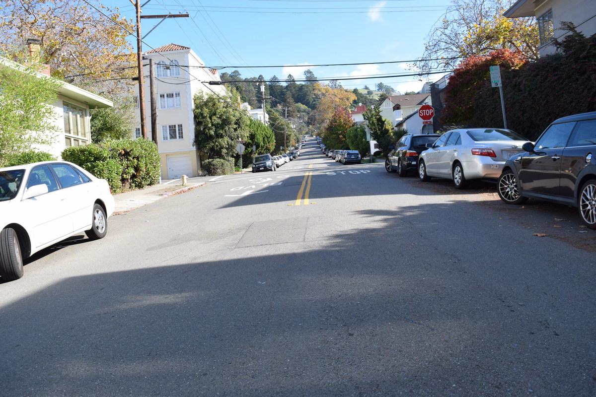
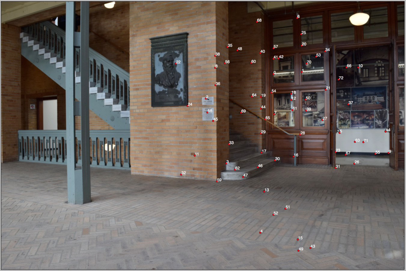
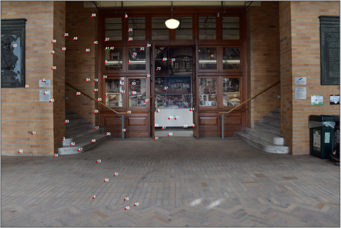
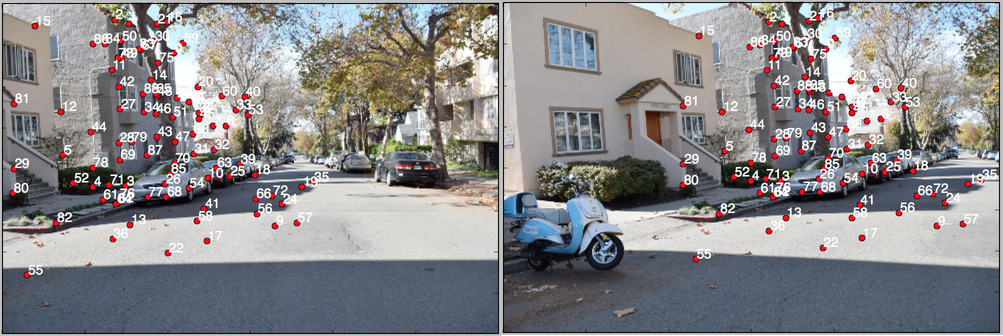
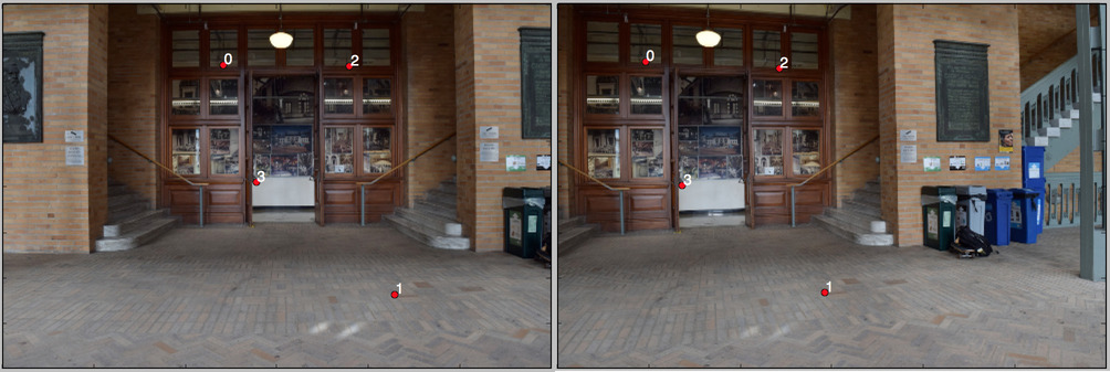
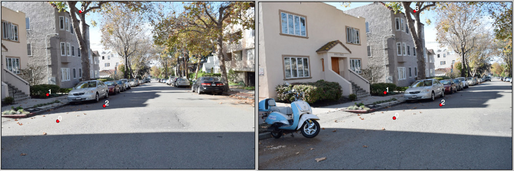
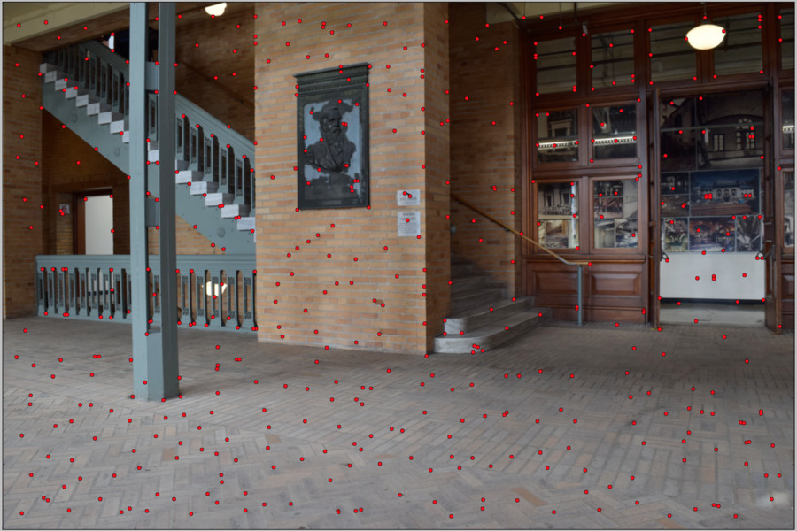
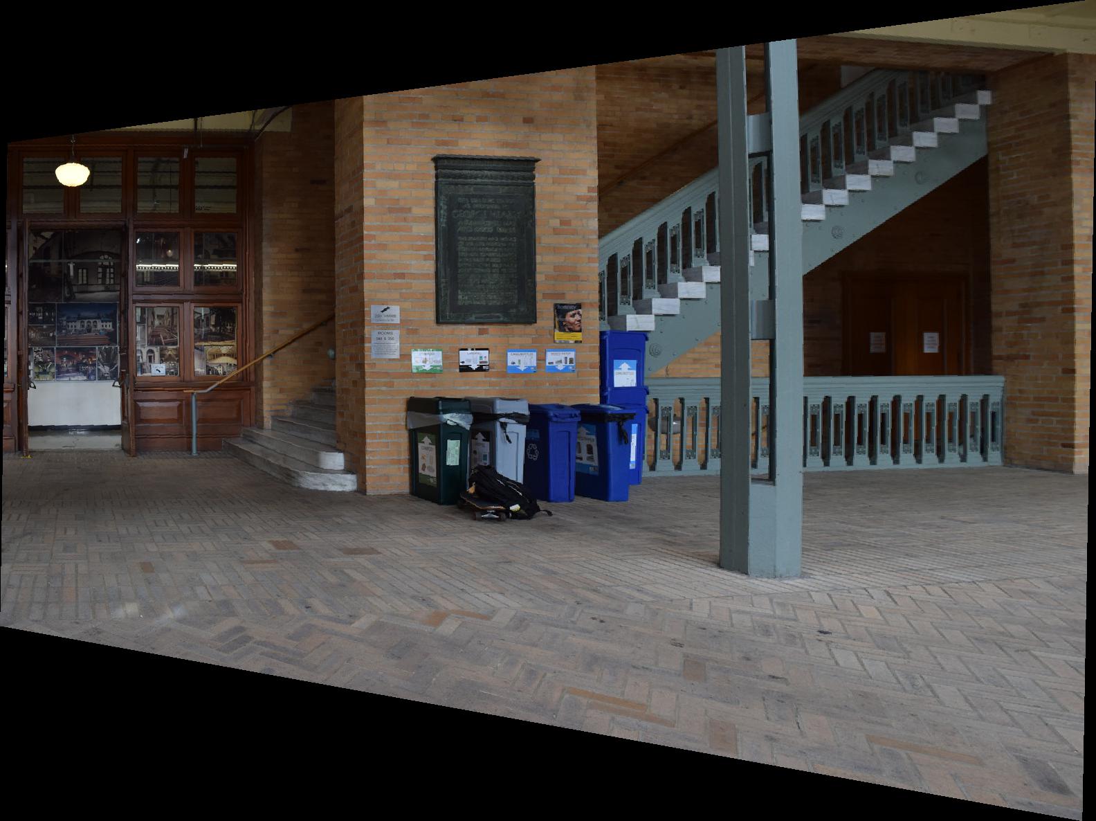
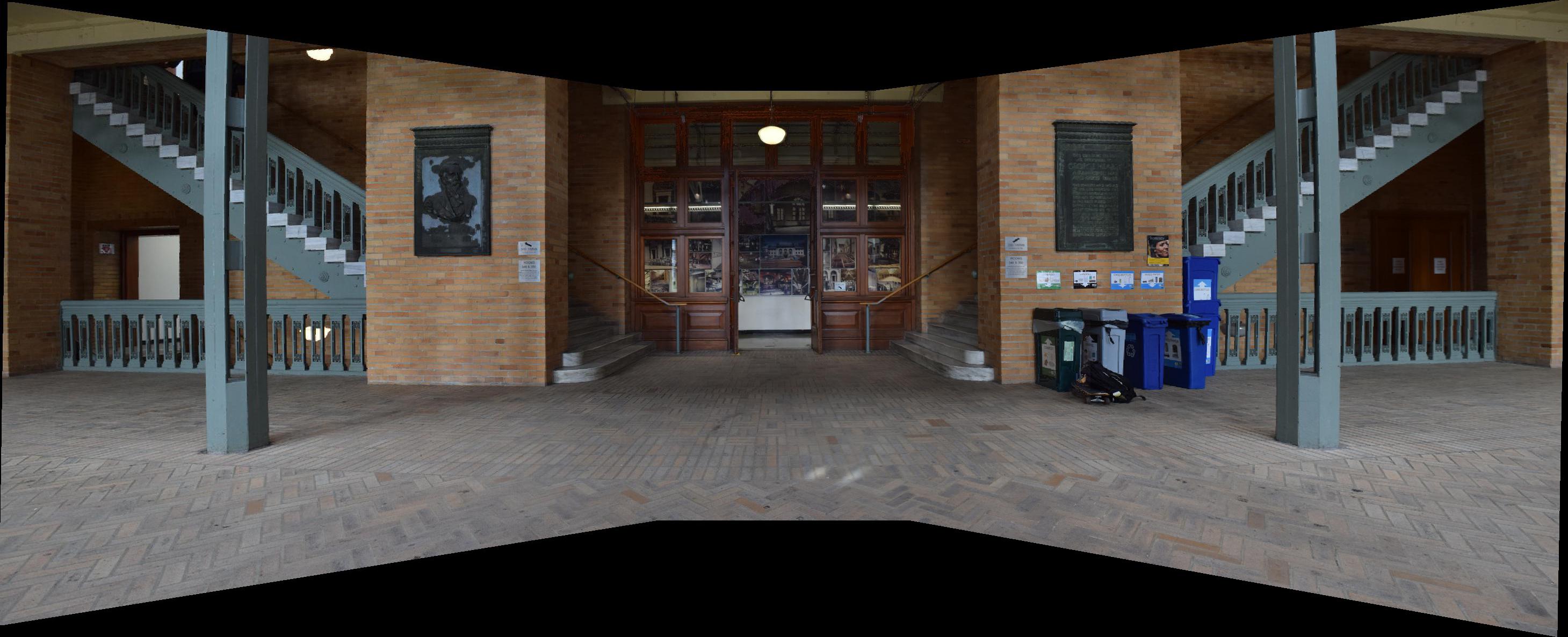
We can take the ideas from part 1 and further apply them to create panorama images. In this case, we must capture images by rotating the camera in such a way that any pair of side by side images has some overlapping features. We can then select the same features in both images in order to transform one image into the shape of the other. Here is an example of the feature selection:

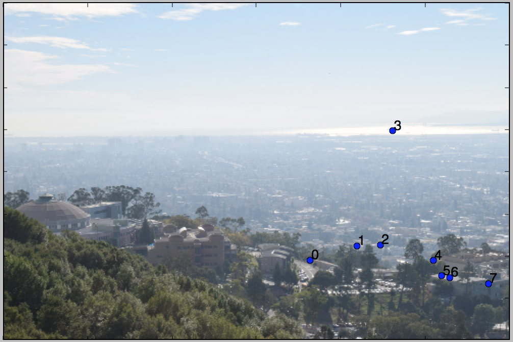
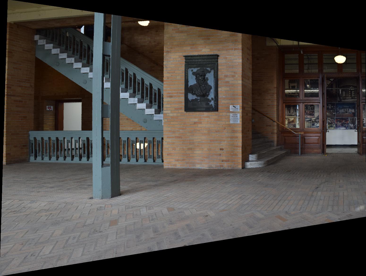
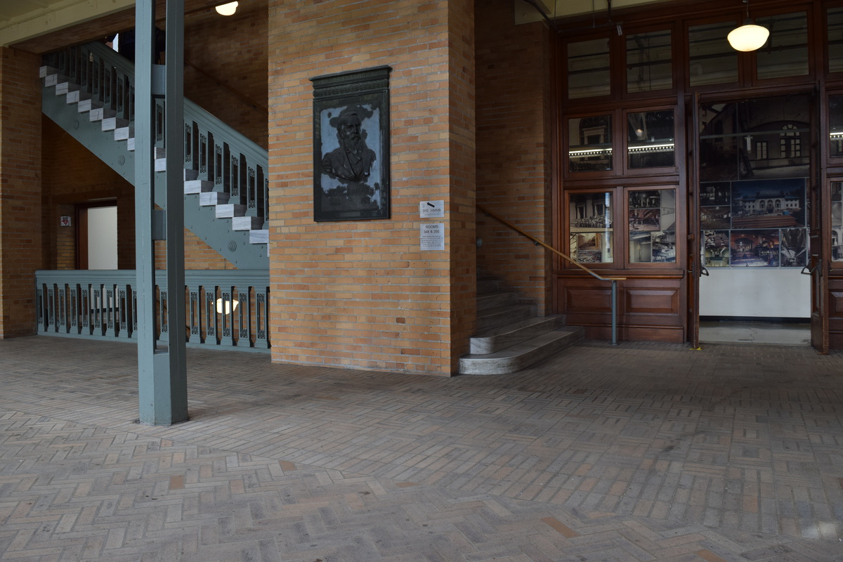
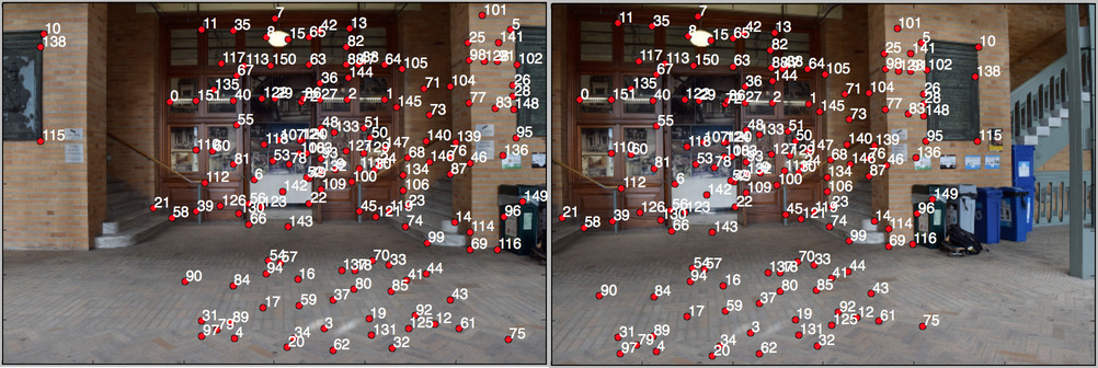
Feature Points of Left Panel

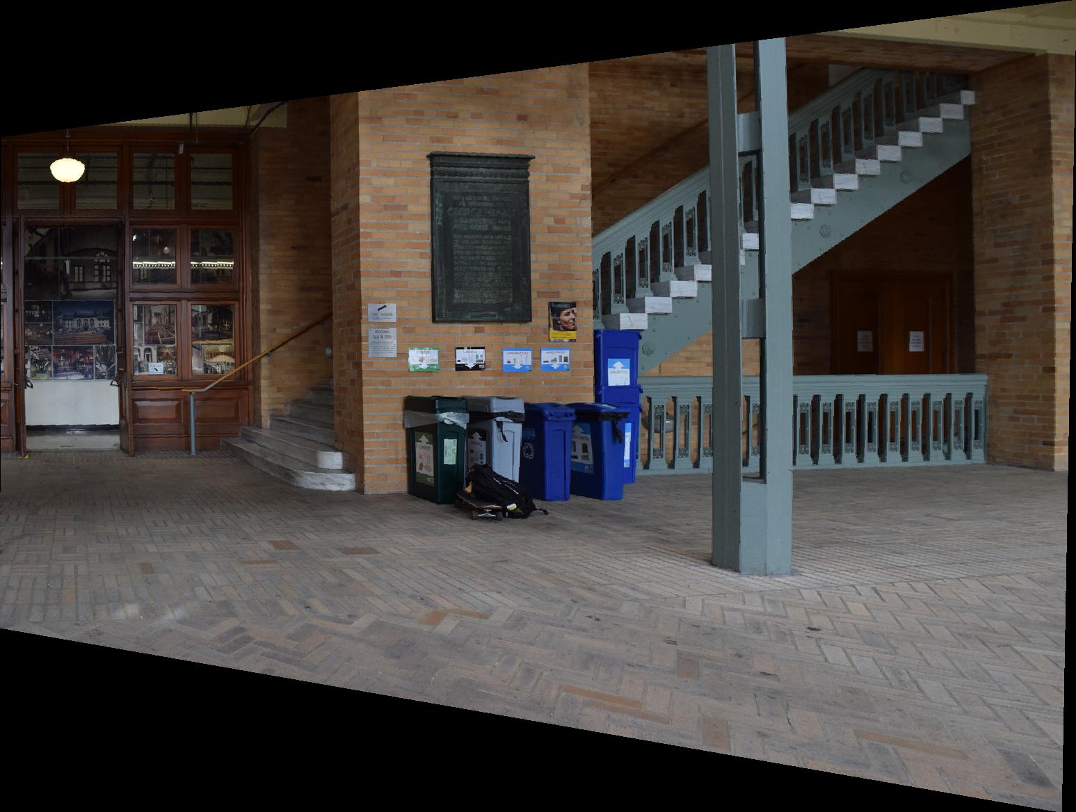
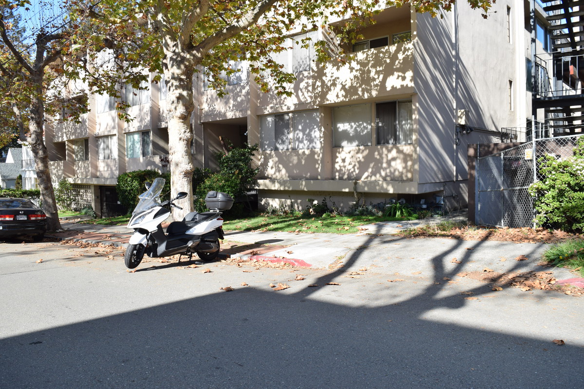
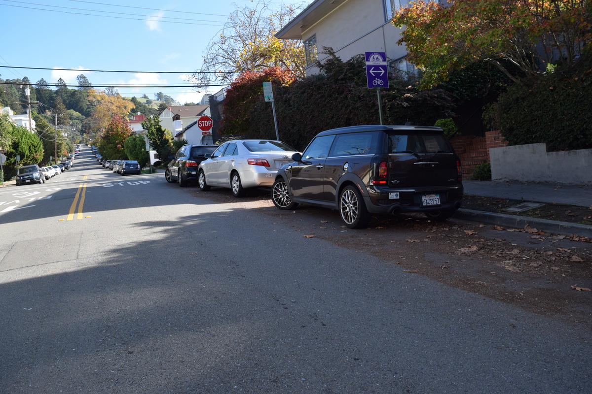
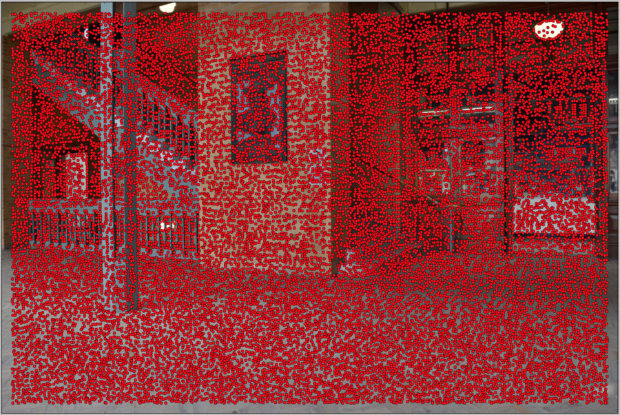
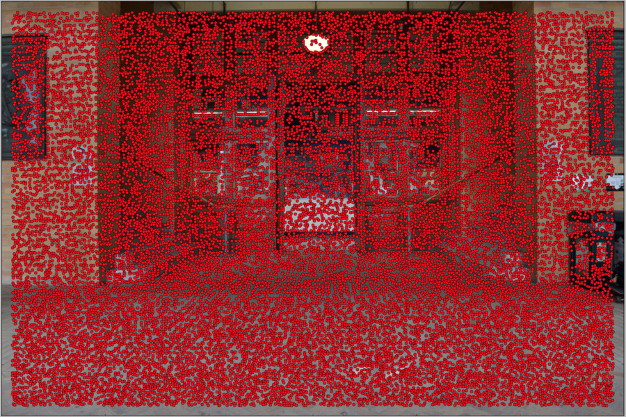
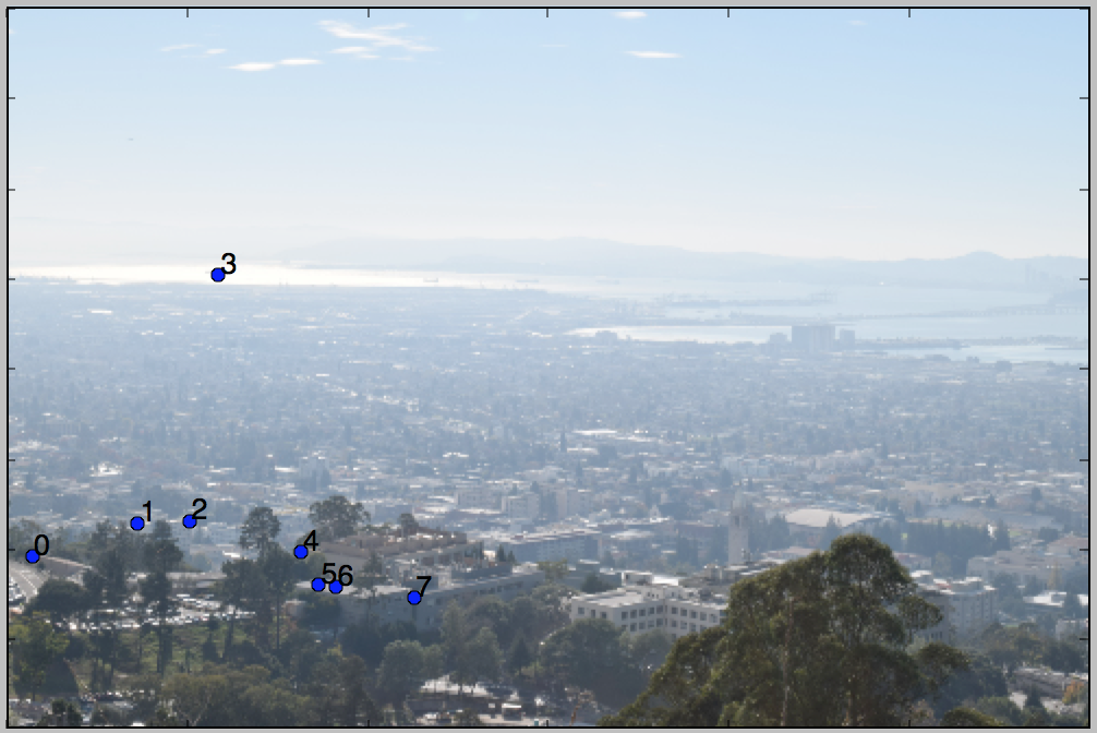
Feature Points of Center Panel

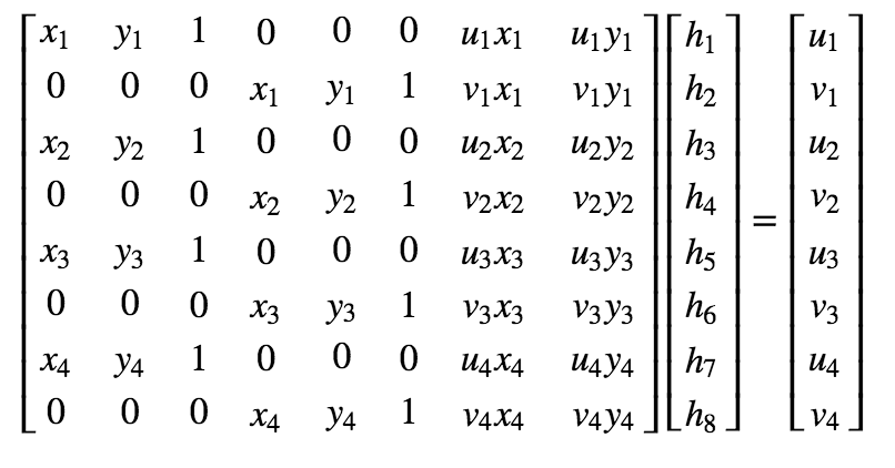
Note that I selected more than 4 feature points this time. This is because overconstraining the system of equations is actually beneficial. The overall algorithm is extremely prone to human error in choosing feature points. A small error can make the transformation drastically different and for this reason, we overconstrain the system with 8 pairs of feature points and solve it using the built in least squares solver to mitigate errors of any individual pair of feature points.

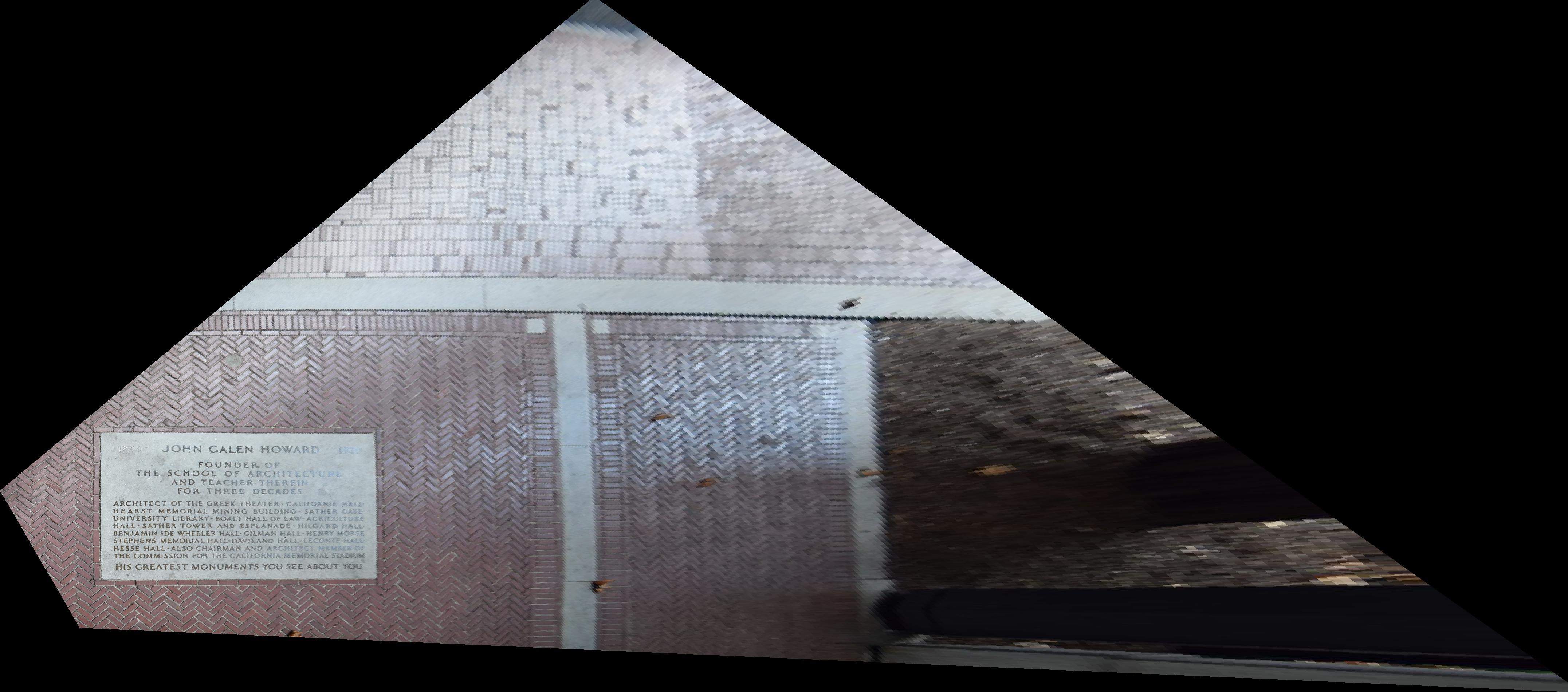
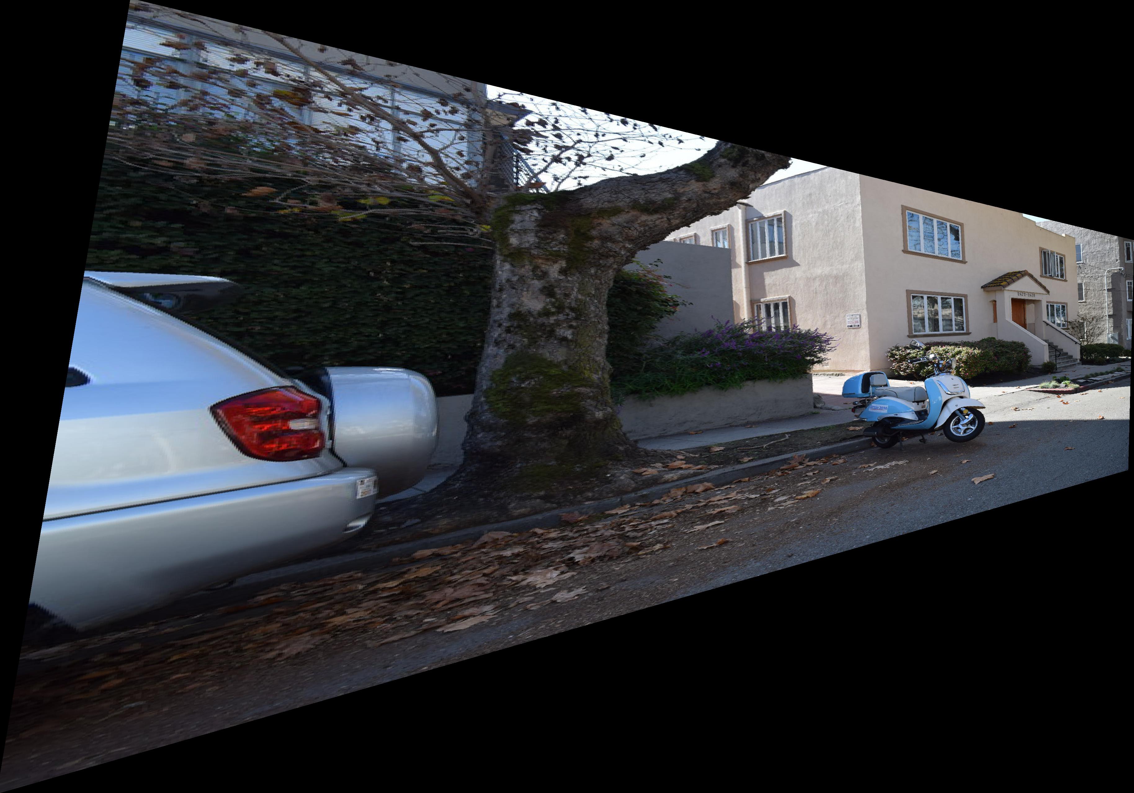
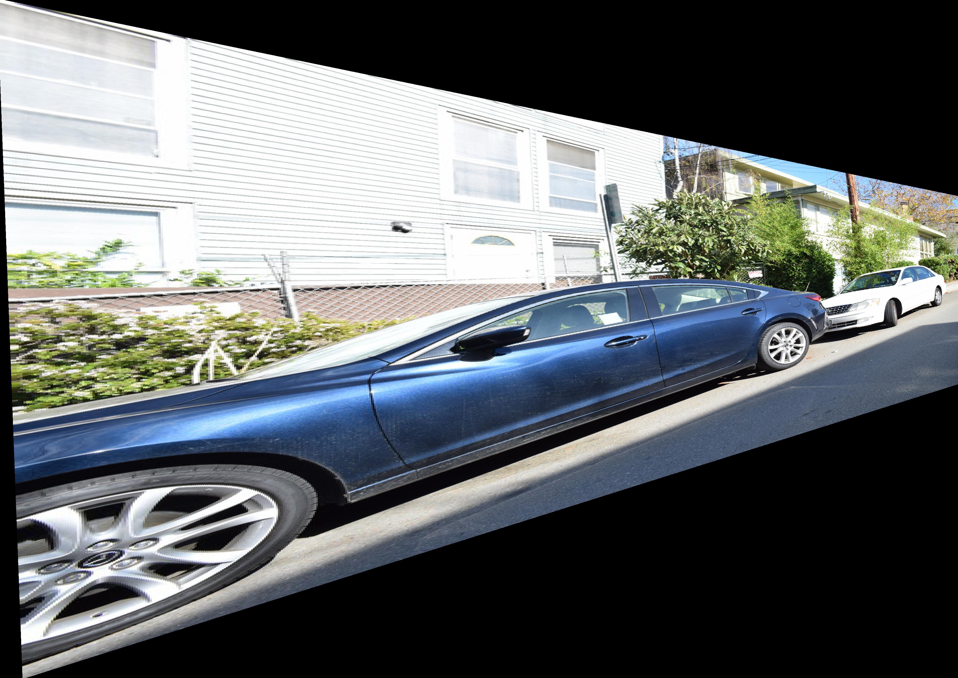
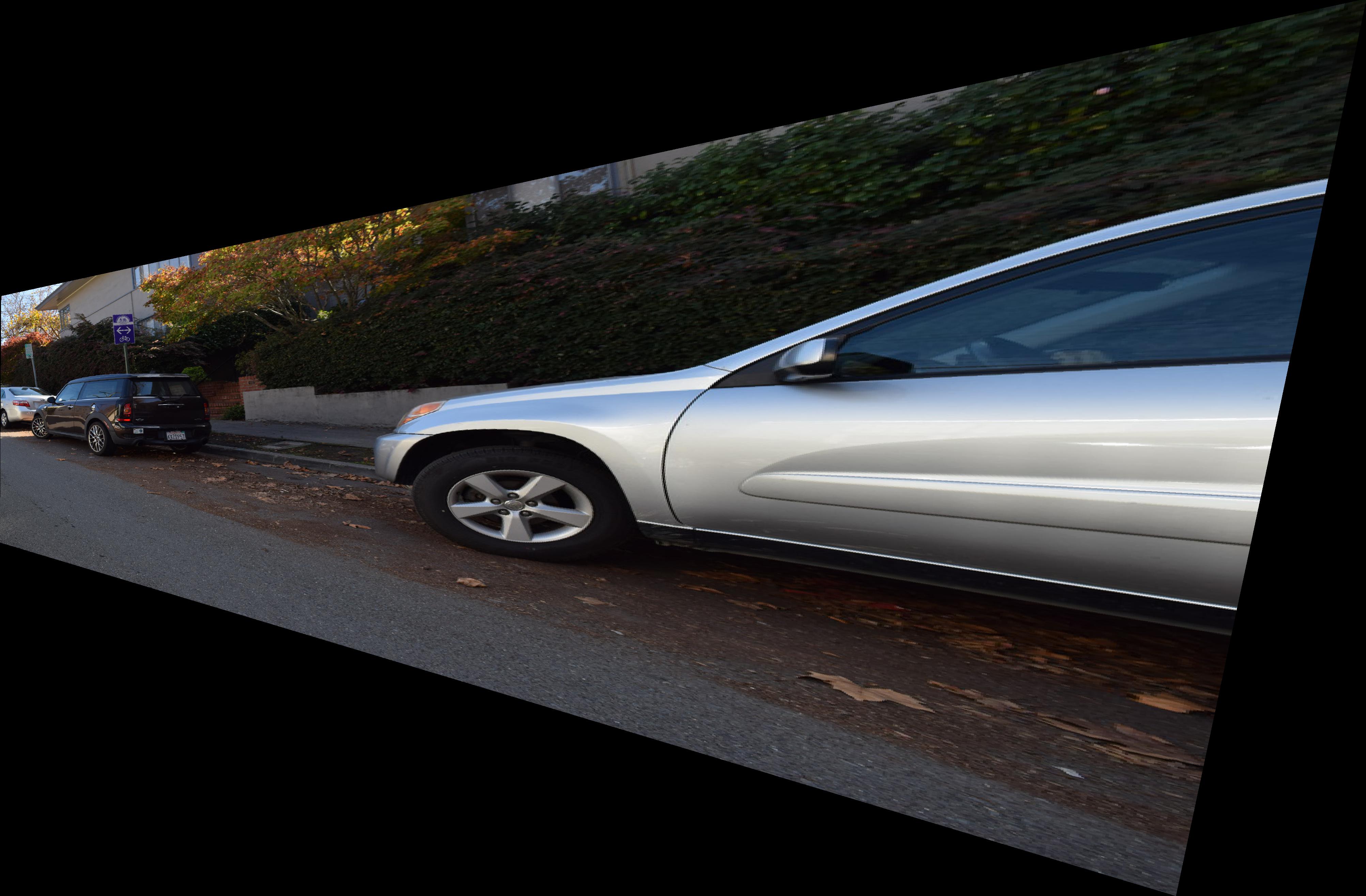
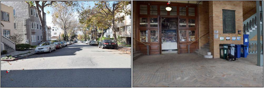
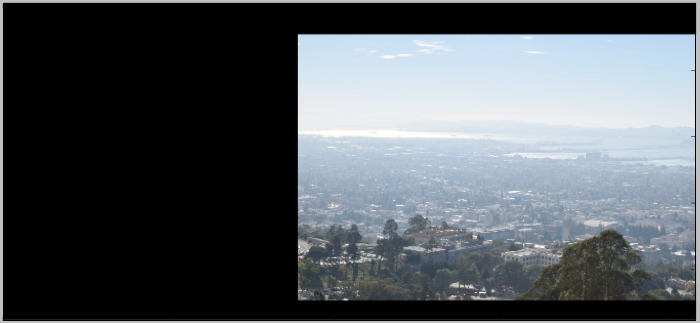
Once we determine the homography matrix H we can inverse warp one image into the shape of the other image as we did in the previous part. In this case, I chose to keep my center panel static and warped my left panel into the center panel's shape:

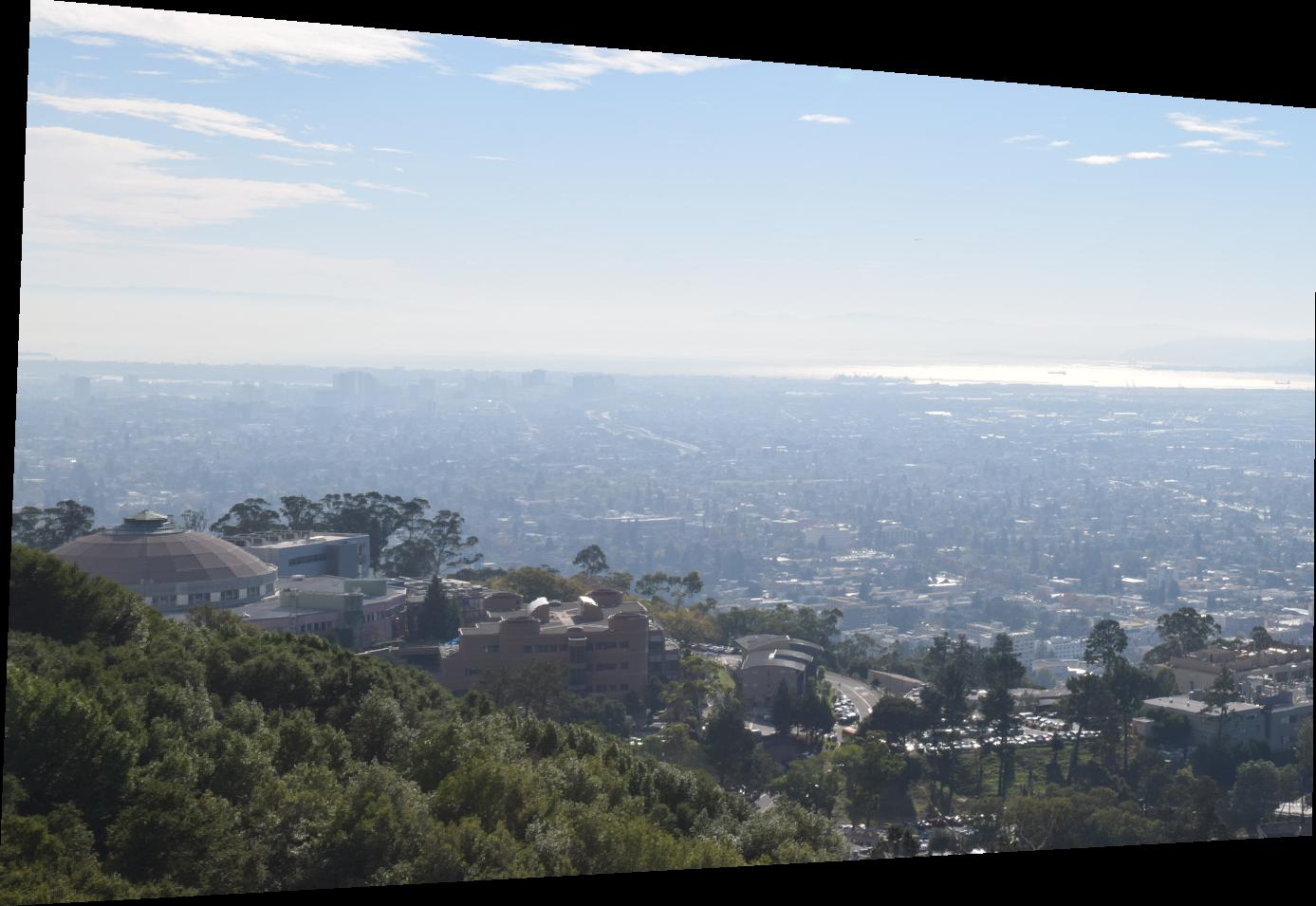
Warped Left Panel

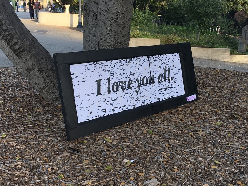
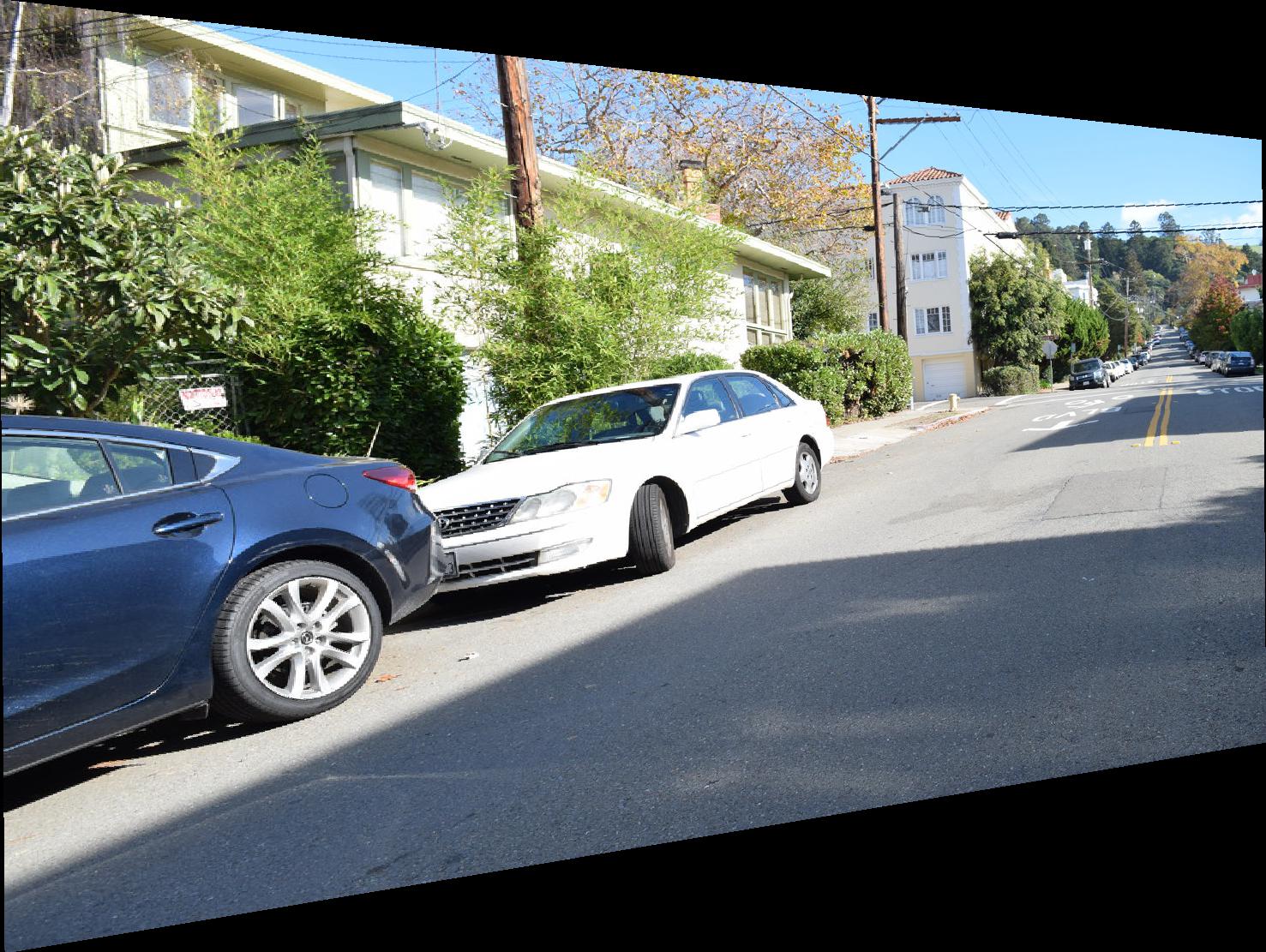
Static Center Panel

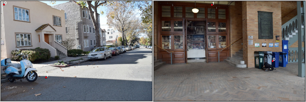
Next, we can gauge the relative locations of the images by comparing the transformed corners of the left panel (the image we are warping) to the coordinates of the original center image. In this way we can offset and align the images properly and furthermore create an output matrix large enough to hold the entire combination of the two images.

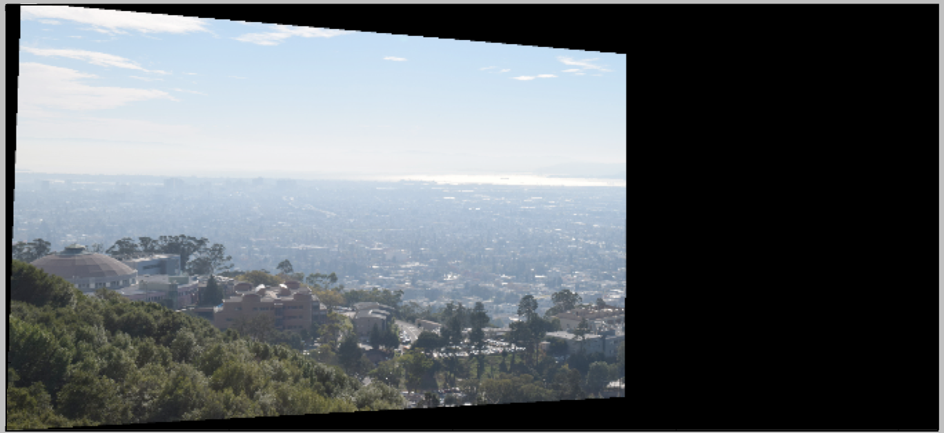
Warped Left Panel

Static Center Panel

There will inevitably be overlap in the two images since there was overlap in the original pair of images. In order to remedy the overlap, we use a linear alpha-blending technique. We construct an alpha mask for each image such that it linearly drops from 1 to 0 for the image on the left (as x increases) and linearly increases from 0 to 1 for the image on the right (as x increases). We create a pair of canvases that are the same size as the ouput images in addition to a pair of masks that are the same size as the input images. We take each mask and place it in each canvas at the same location as the images above.

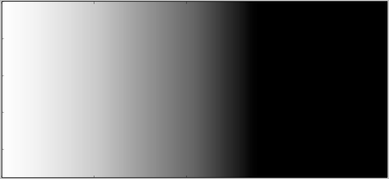
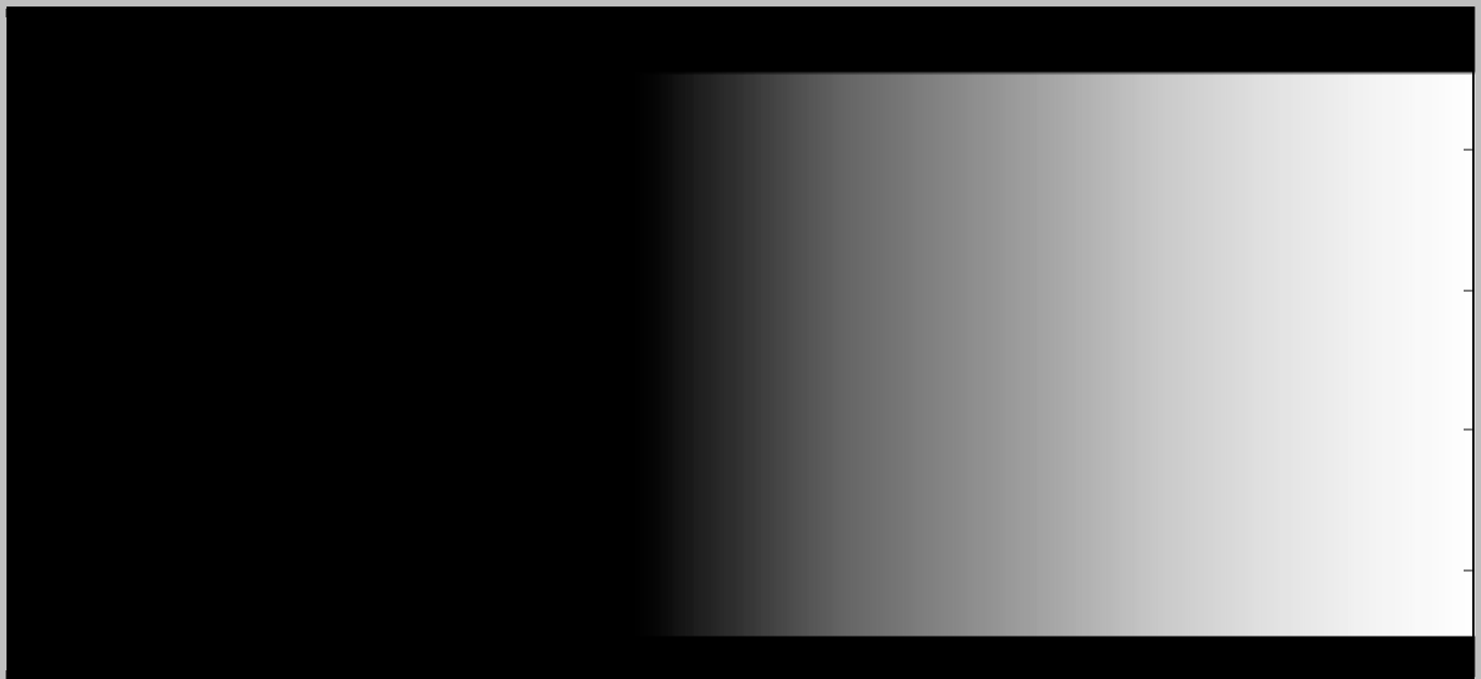
Left Alpha Mask

Center Alpha Mask

We then check to see where the overlap exists. This means we search the images for any location where both images have non-zero pixels. We then run through each of these overlapping pixels and use weighted alpha blending. We check each of the alpha masks for the corresponding alpha value and then determine weights w1 and w2 as follows:

w1 = a1 / (a1 + a2)
w2 = a2 / (a1 + a2)

And finally, we determine the color of the pixel:

output[x, y] = w1 * im1[x, y] + w2 * im2[x, y]

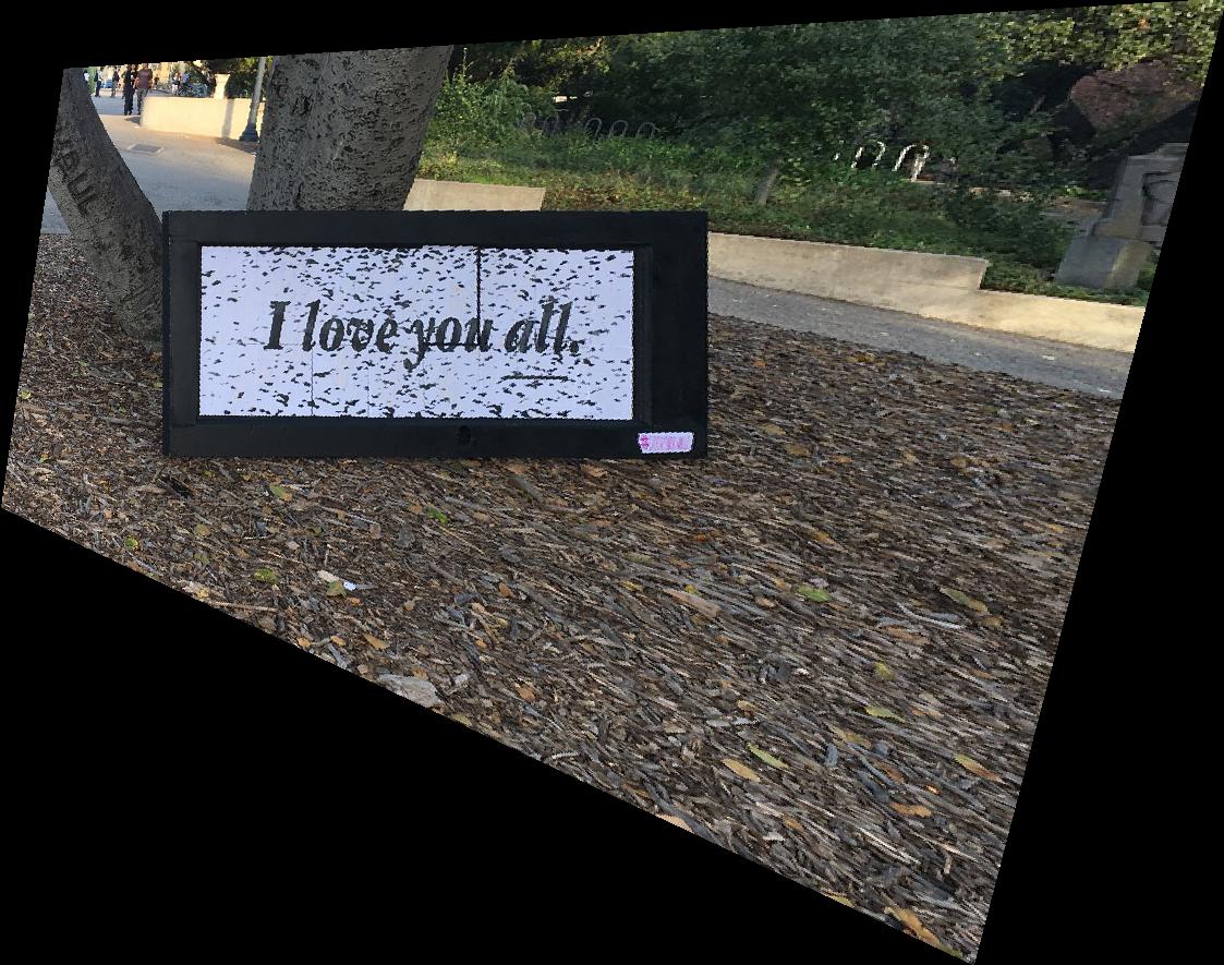
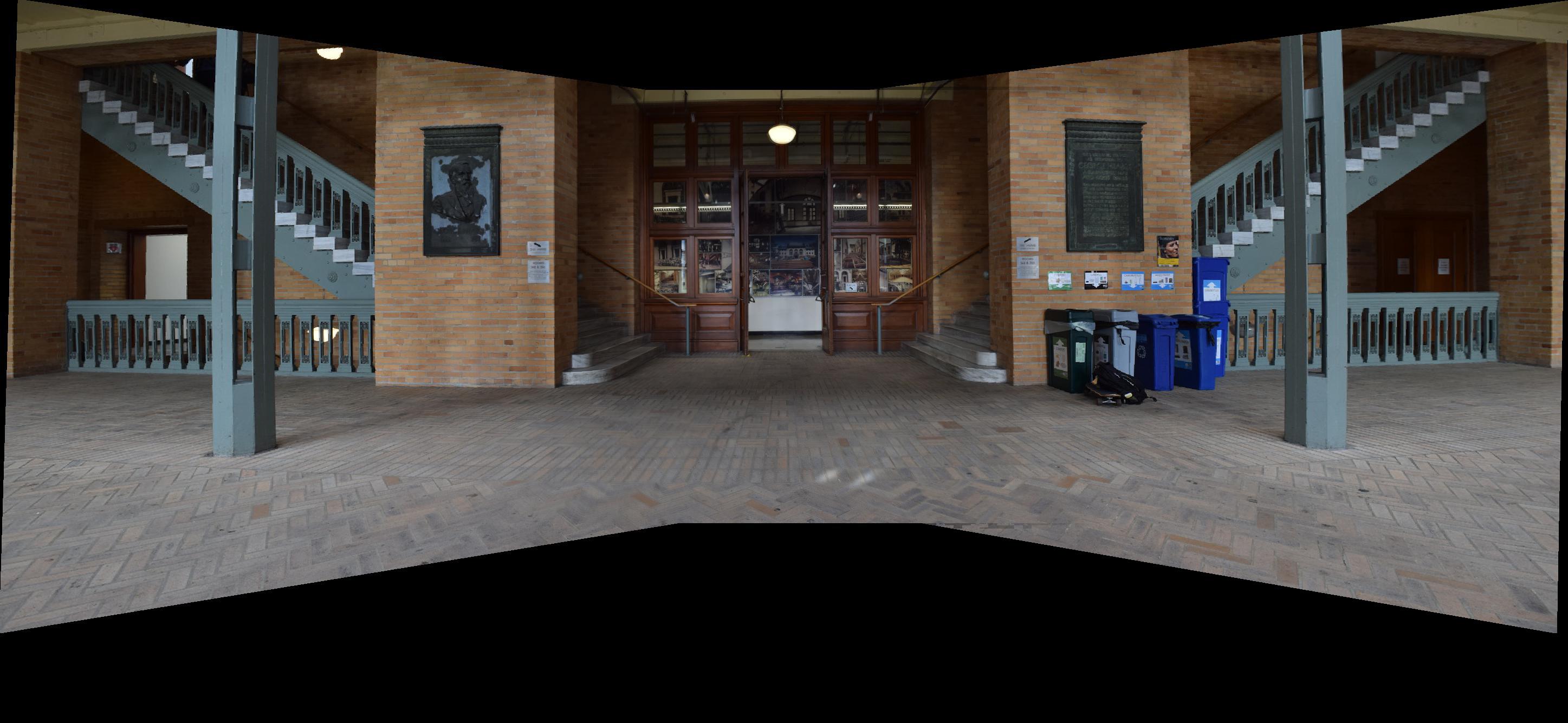
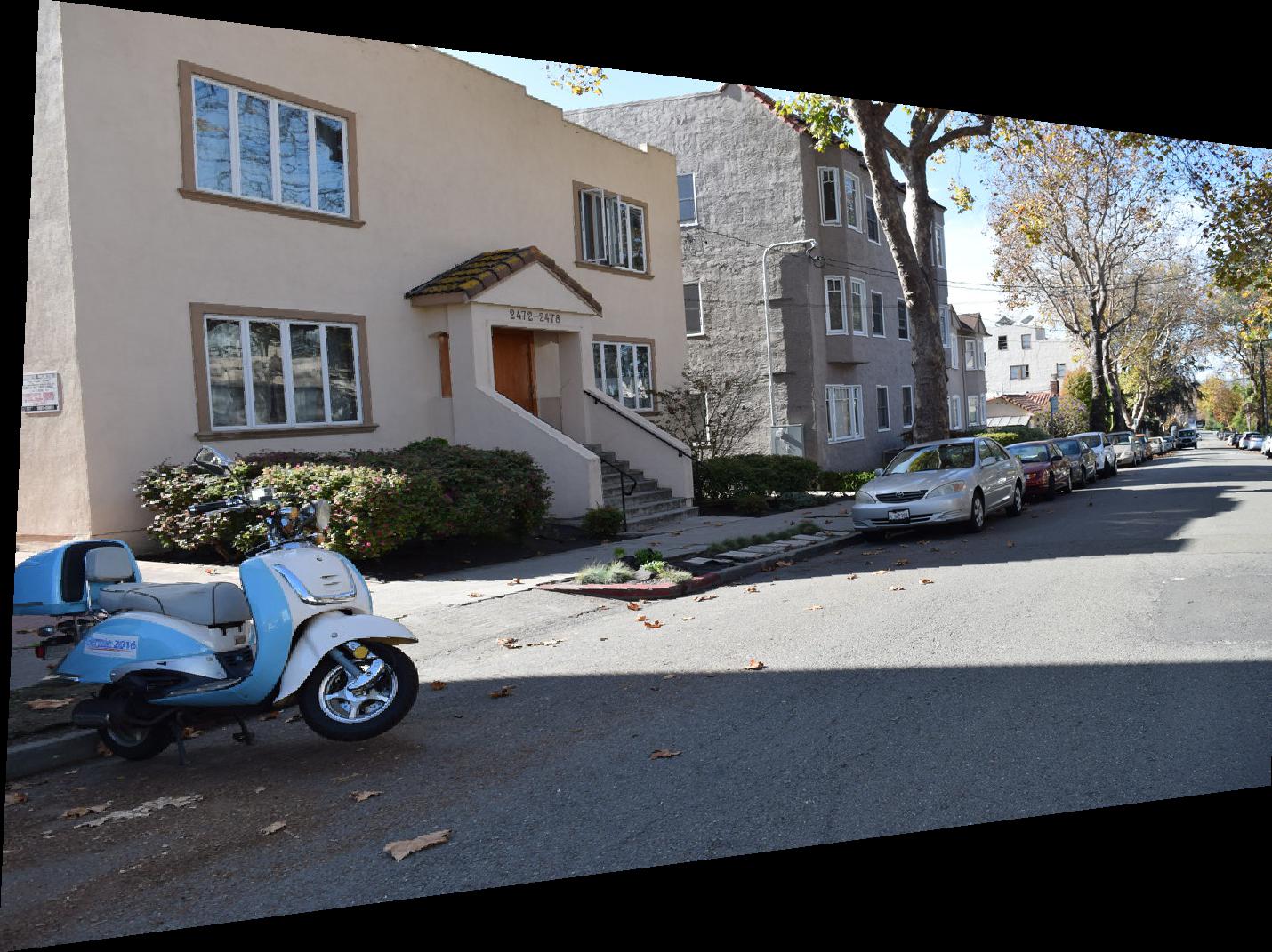
For all non-overlapping pixels, we can simply add the two images together since one or both images will be black. This gets us the following result:

Warped Left and Center Panels after Blending

I attempted to use regular feathering blending on the overlapping borders and laplacian stack blending from our previous project however this method seemed to provide the best results while minimizing artifacting and faded seams. If we want to create a 3 panel panorama, we can take our output image, treat it as the static fixed image, and then warp another image into its shape.

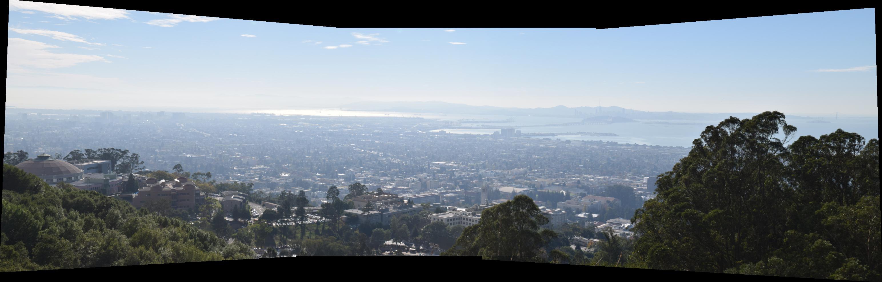
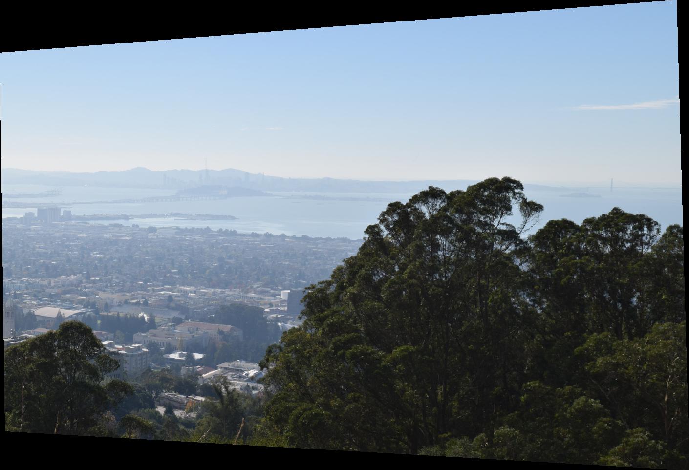
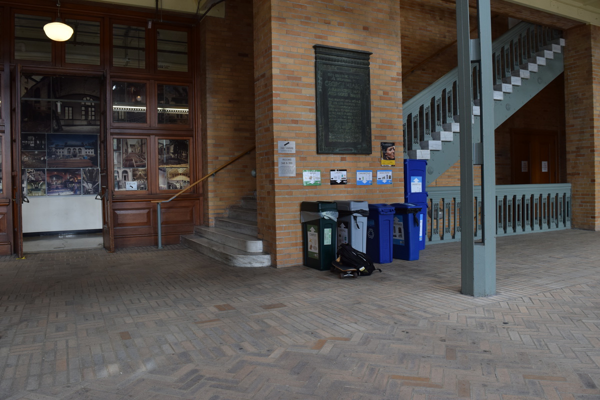
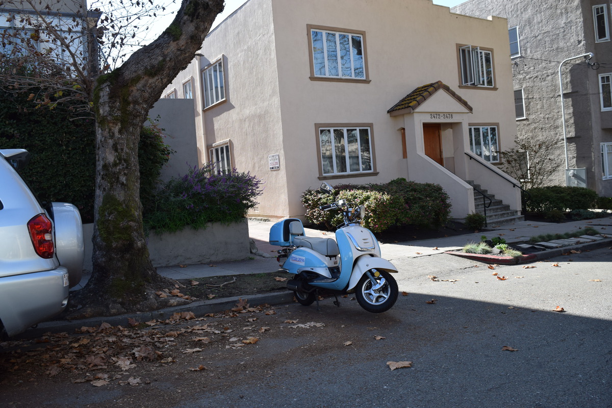
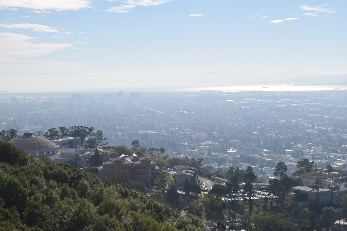
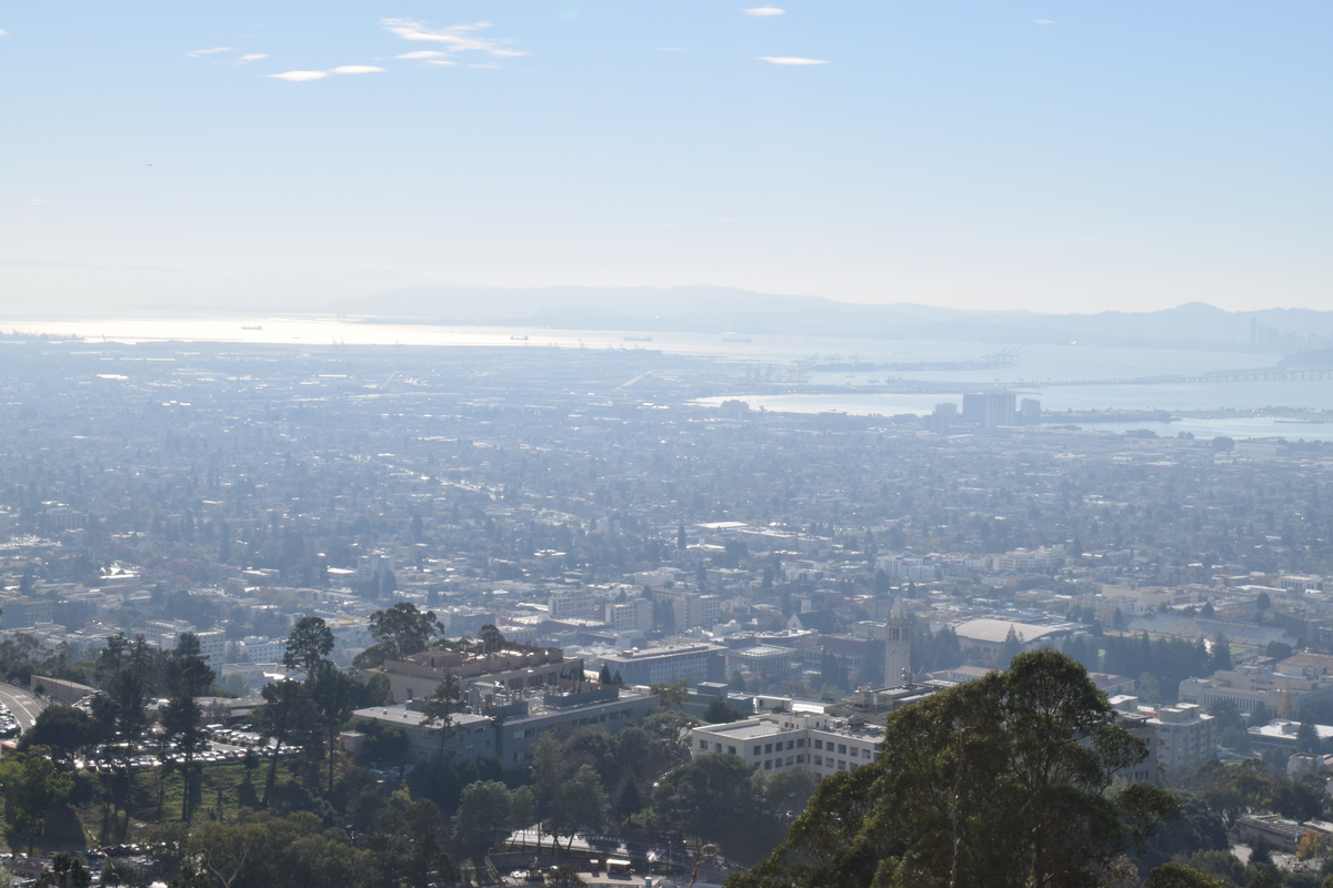
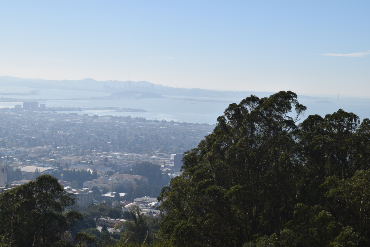
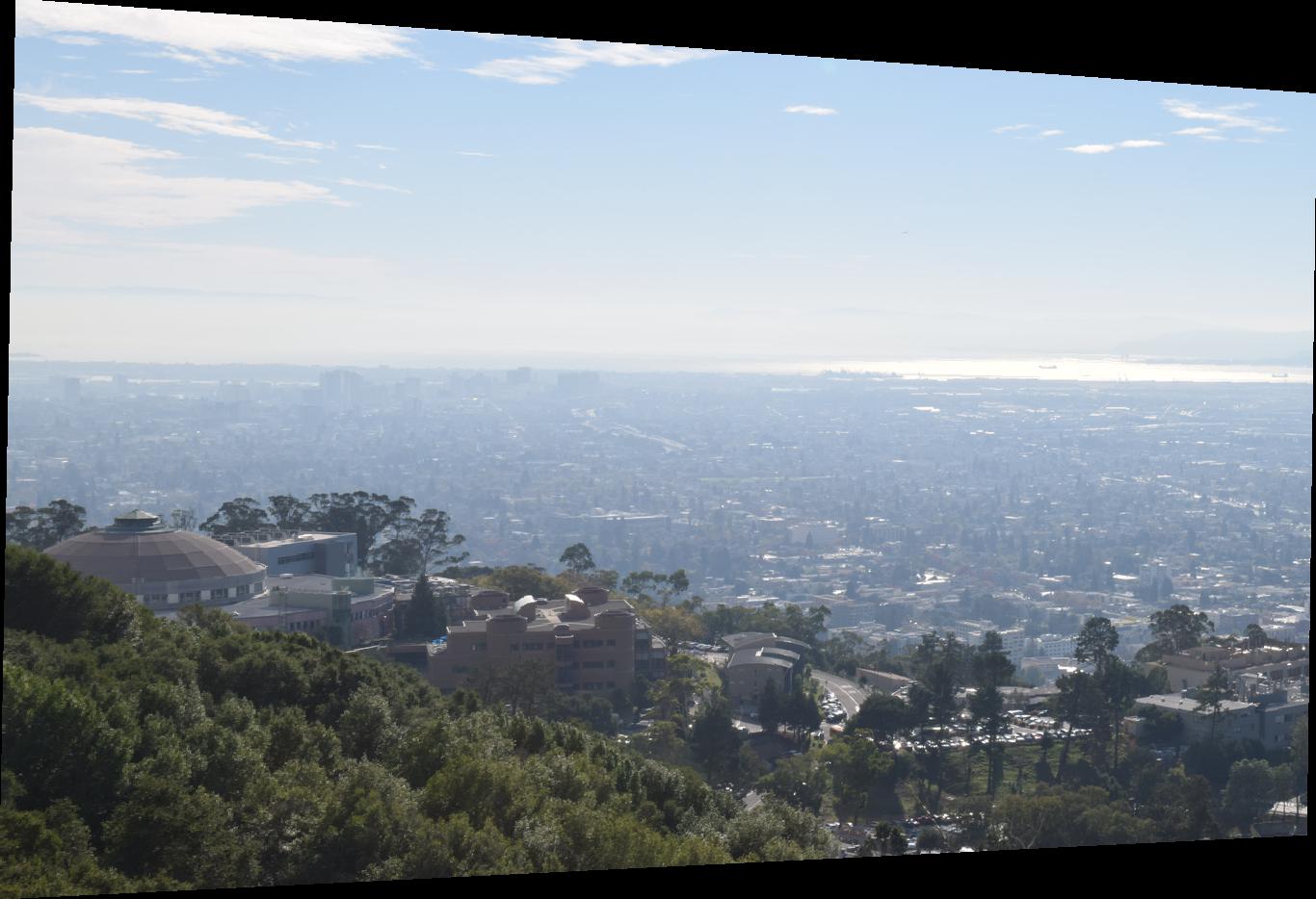
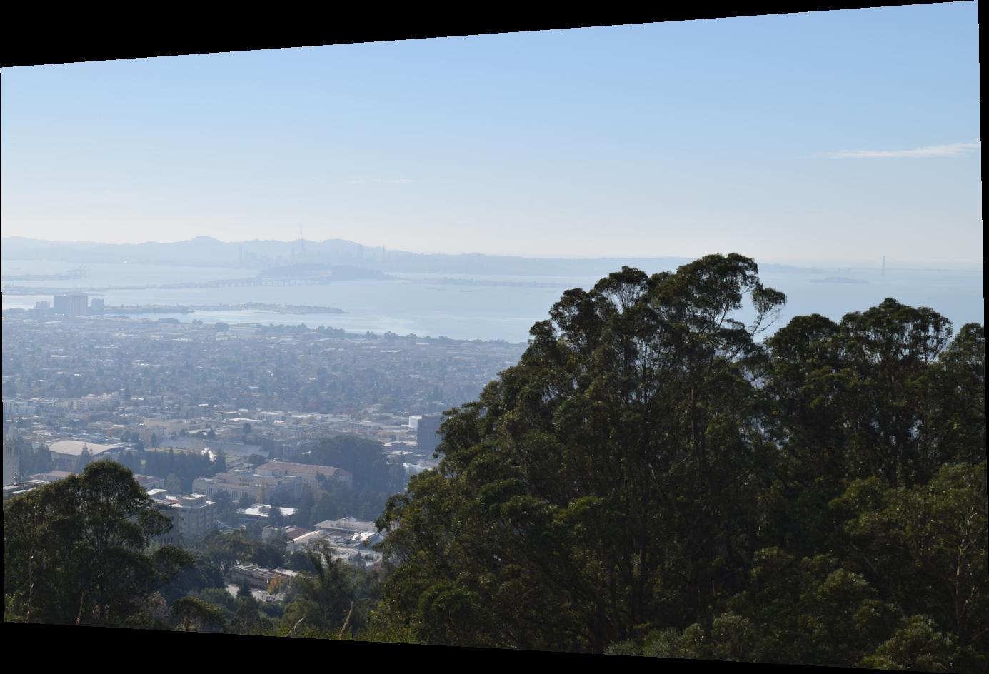
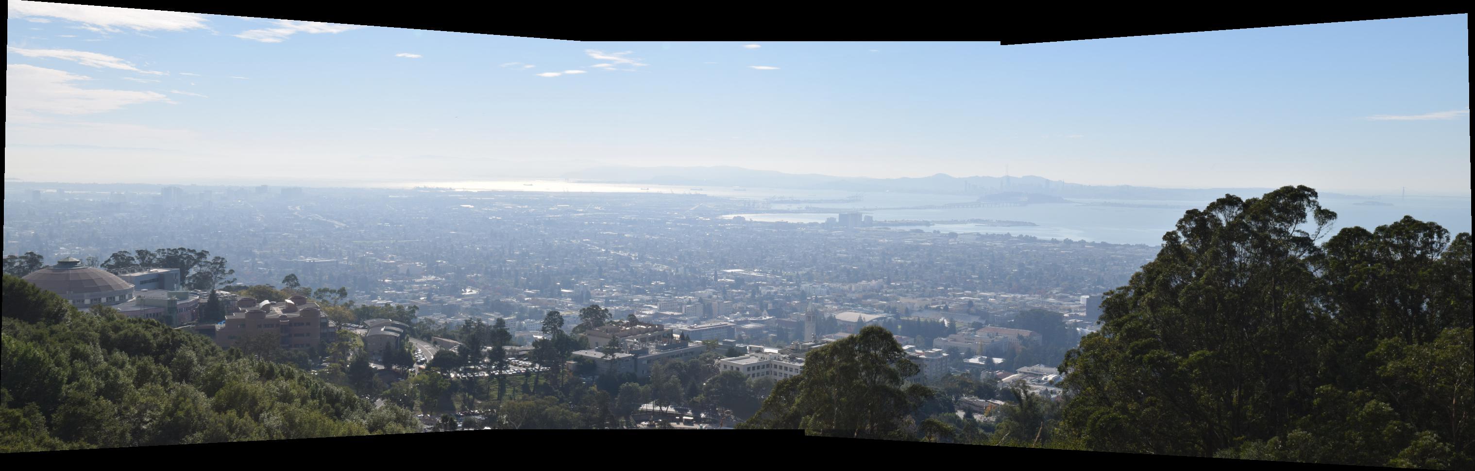
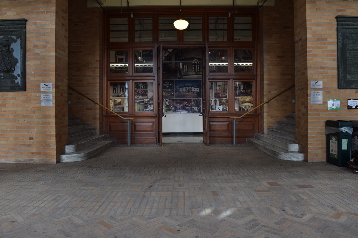
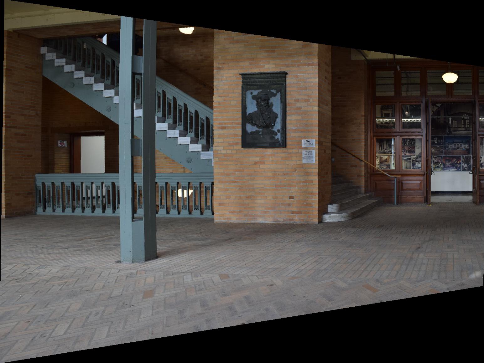
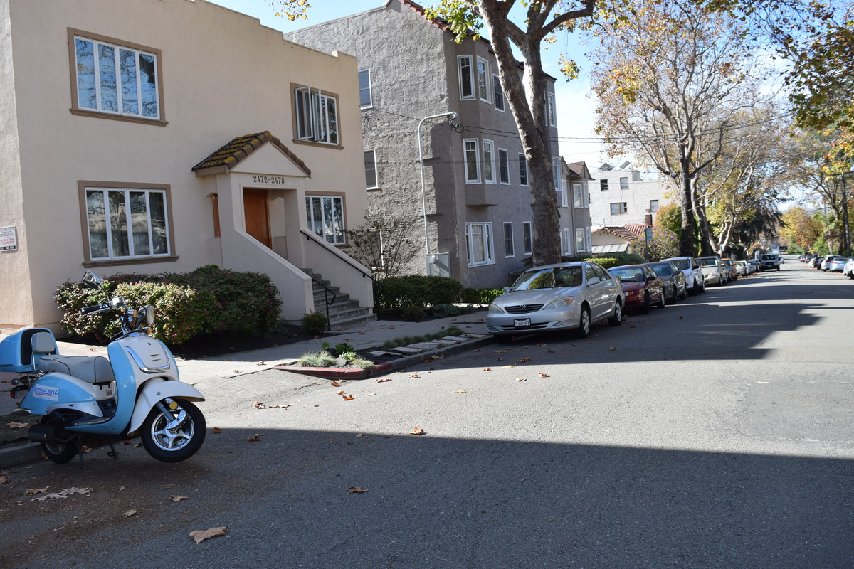
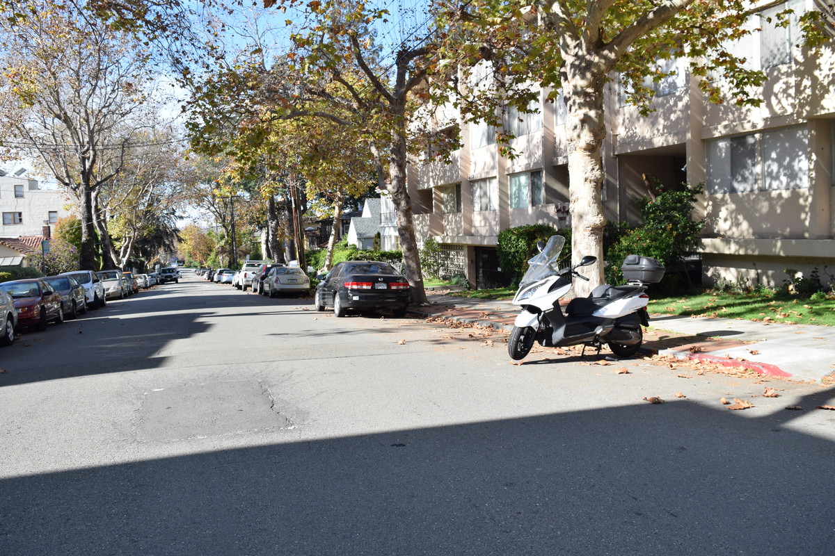
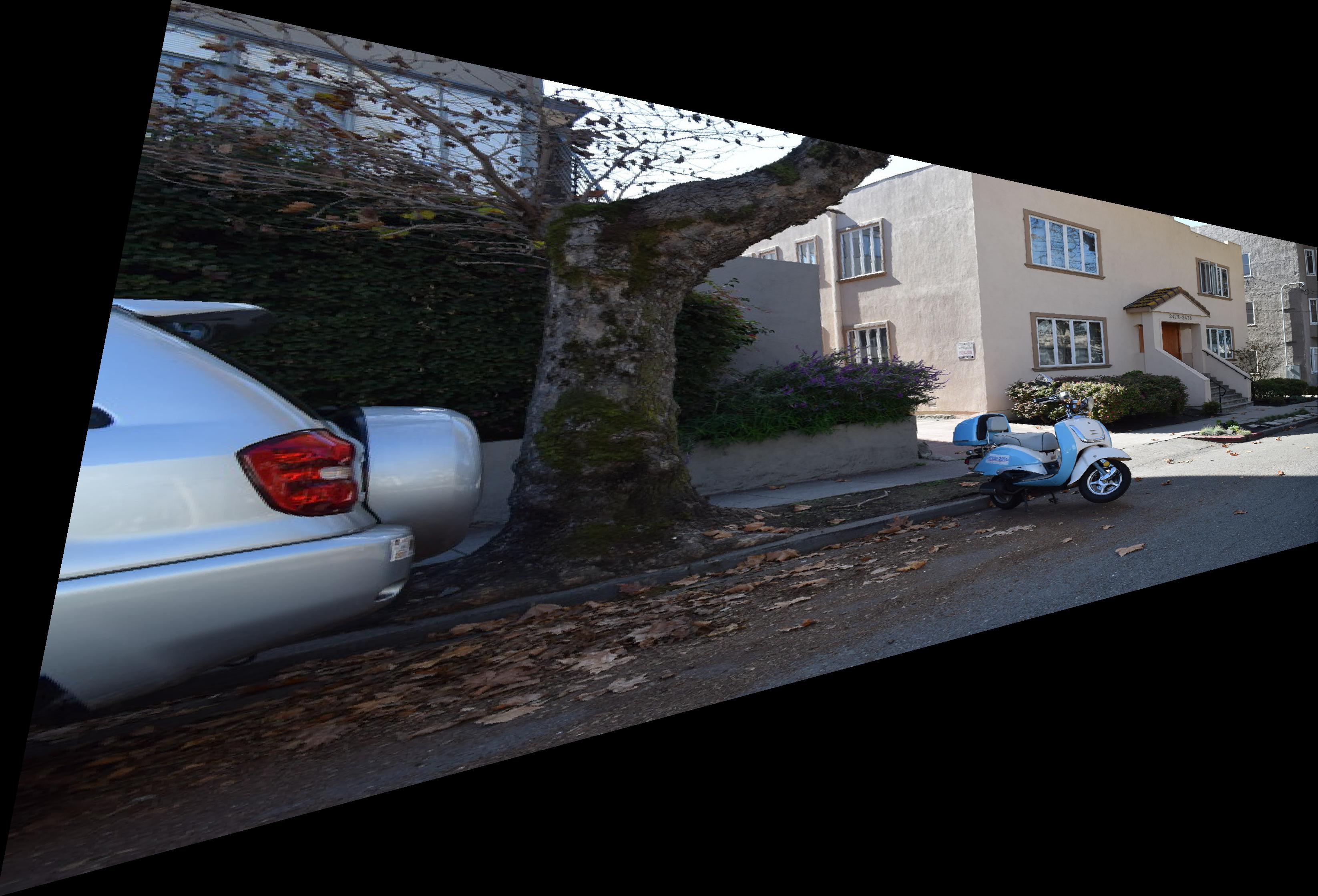
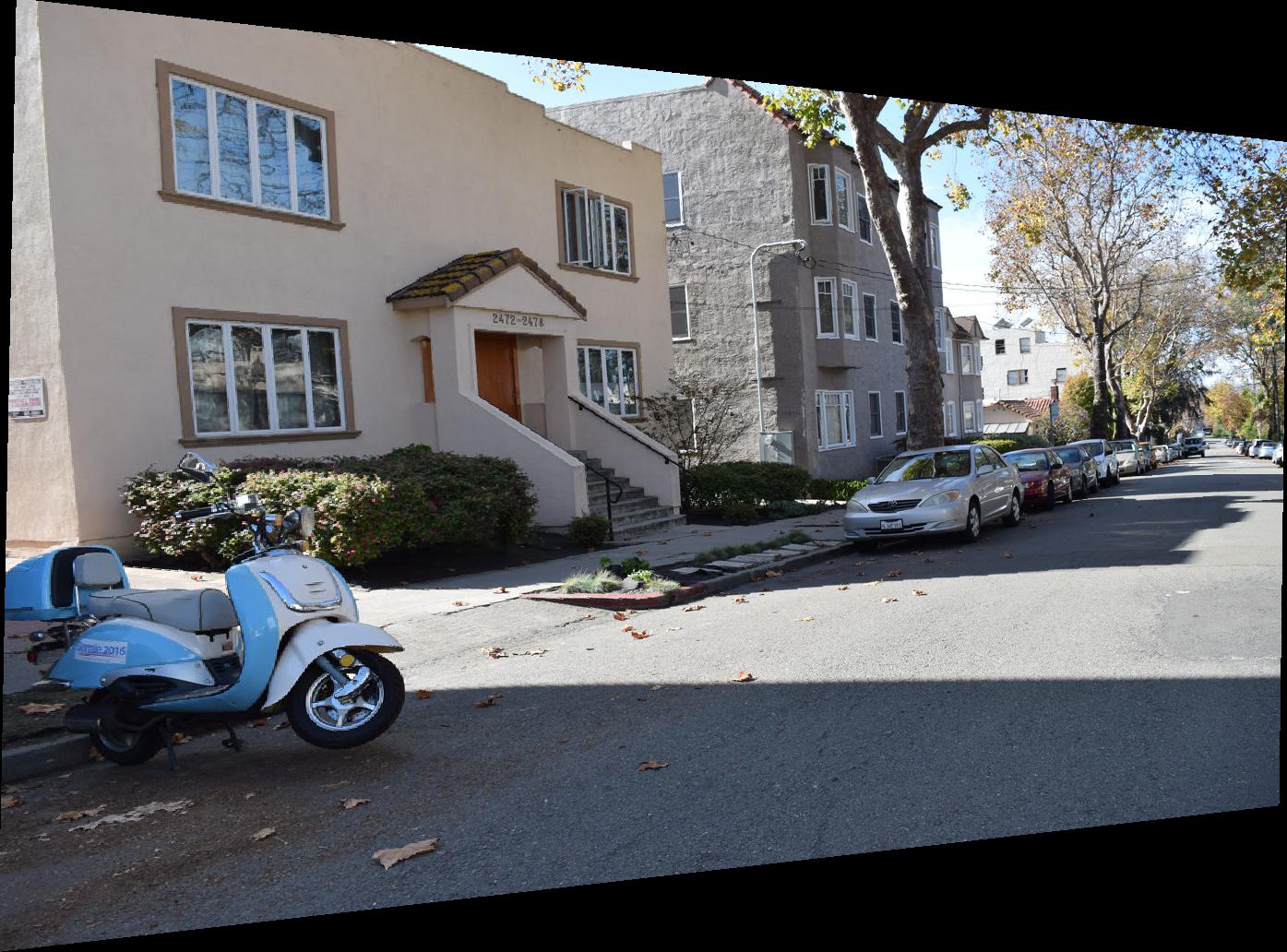
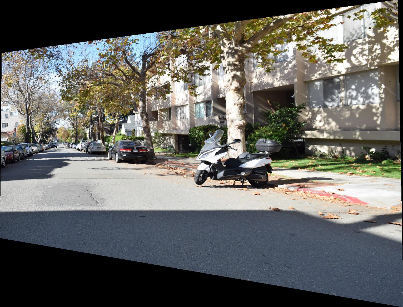
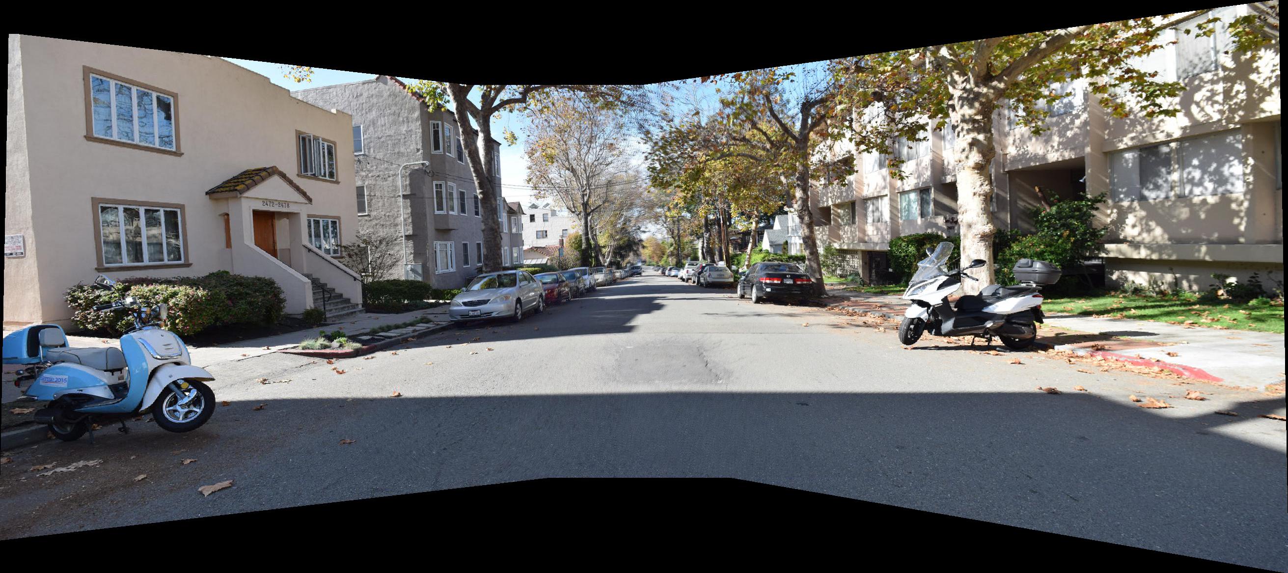
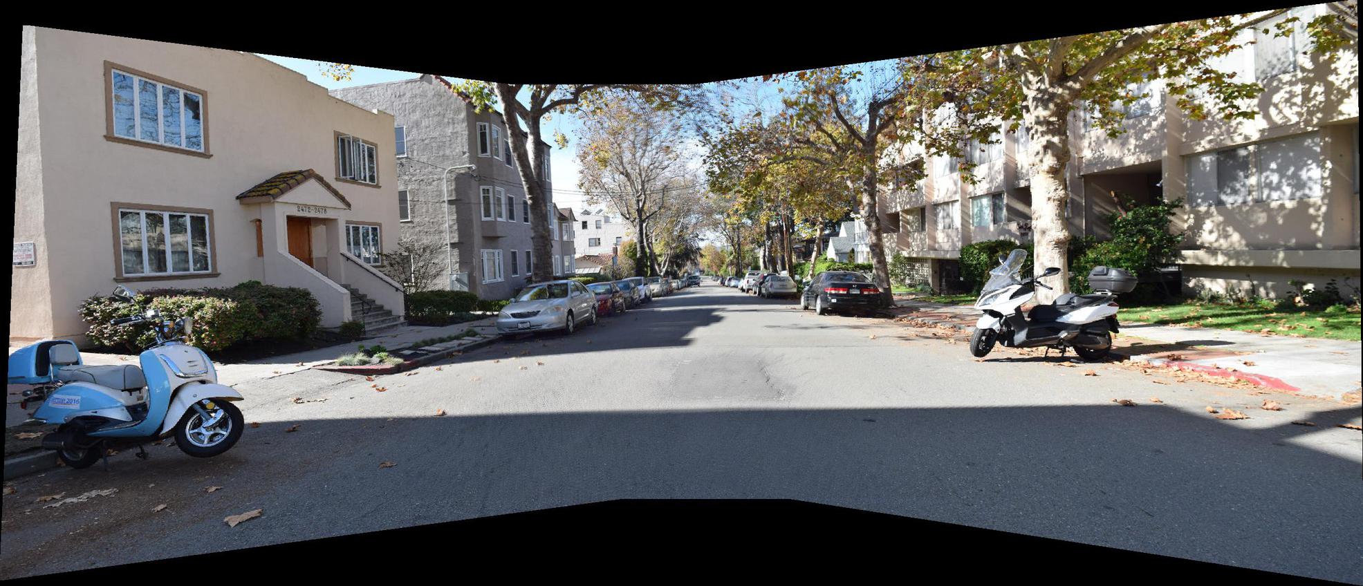
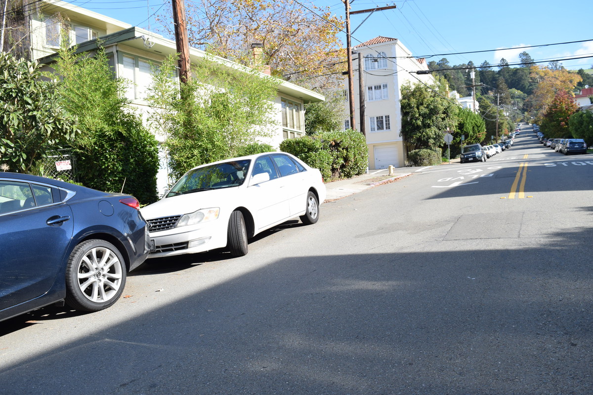
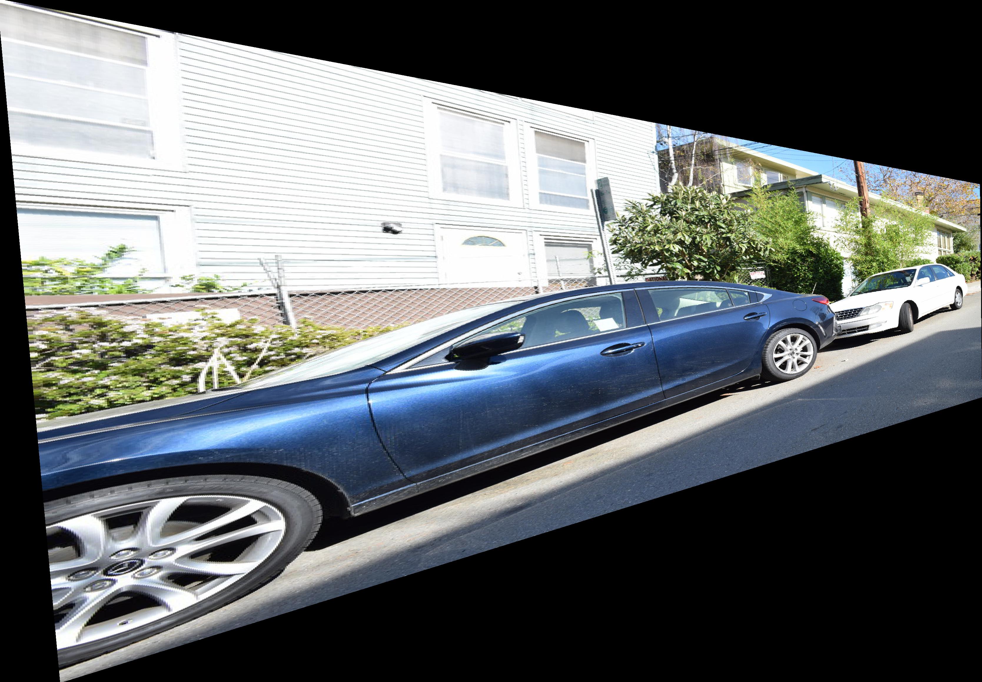
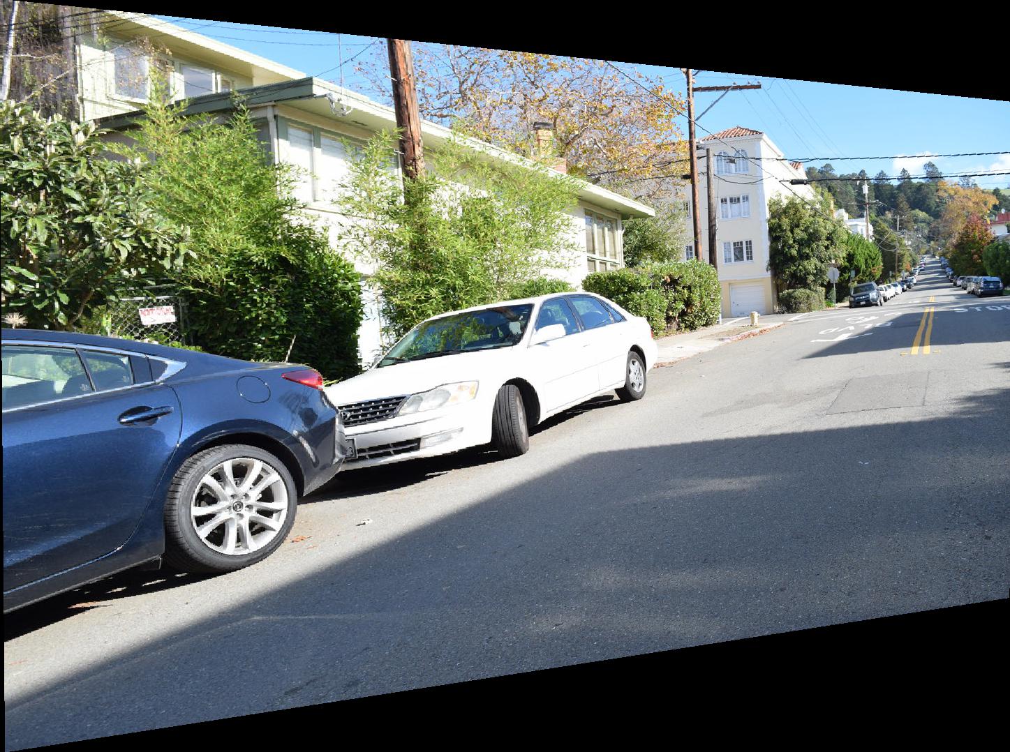
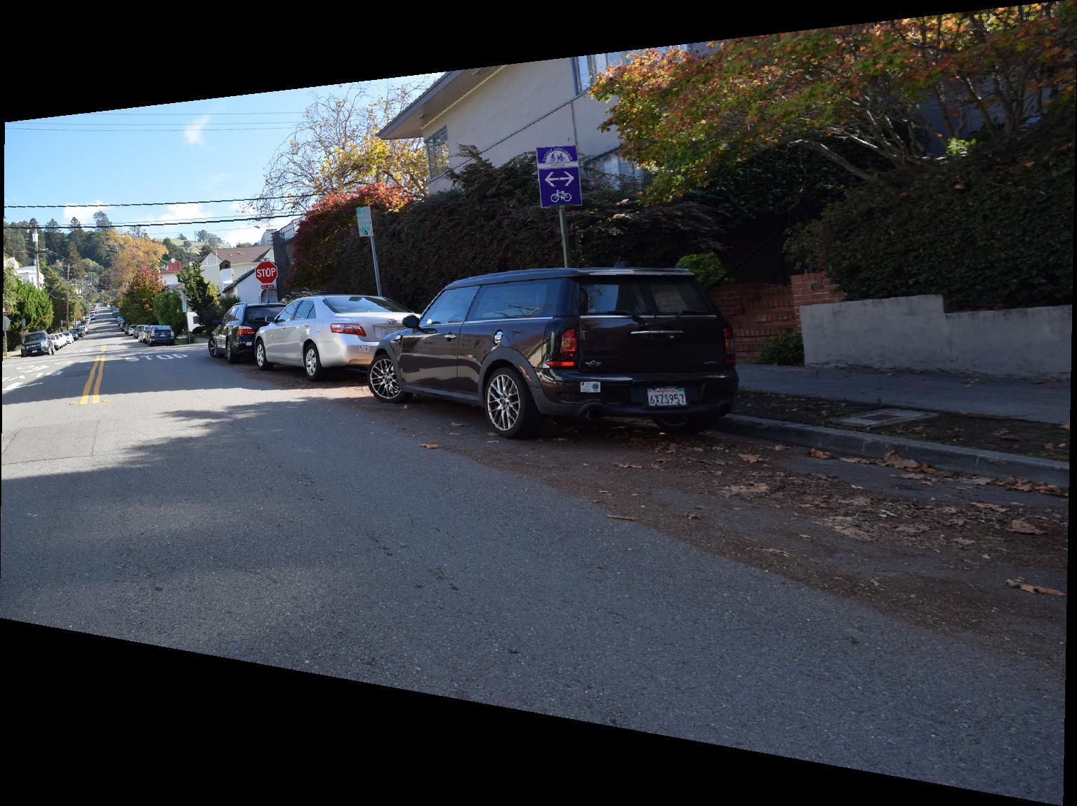
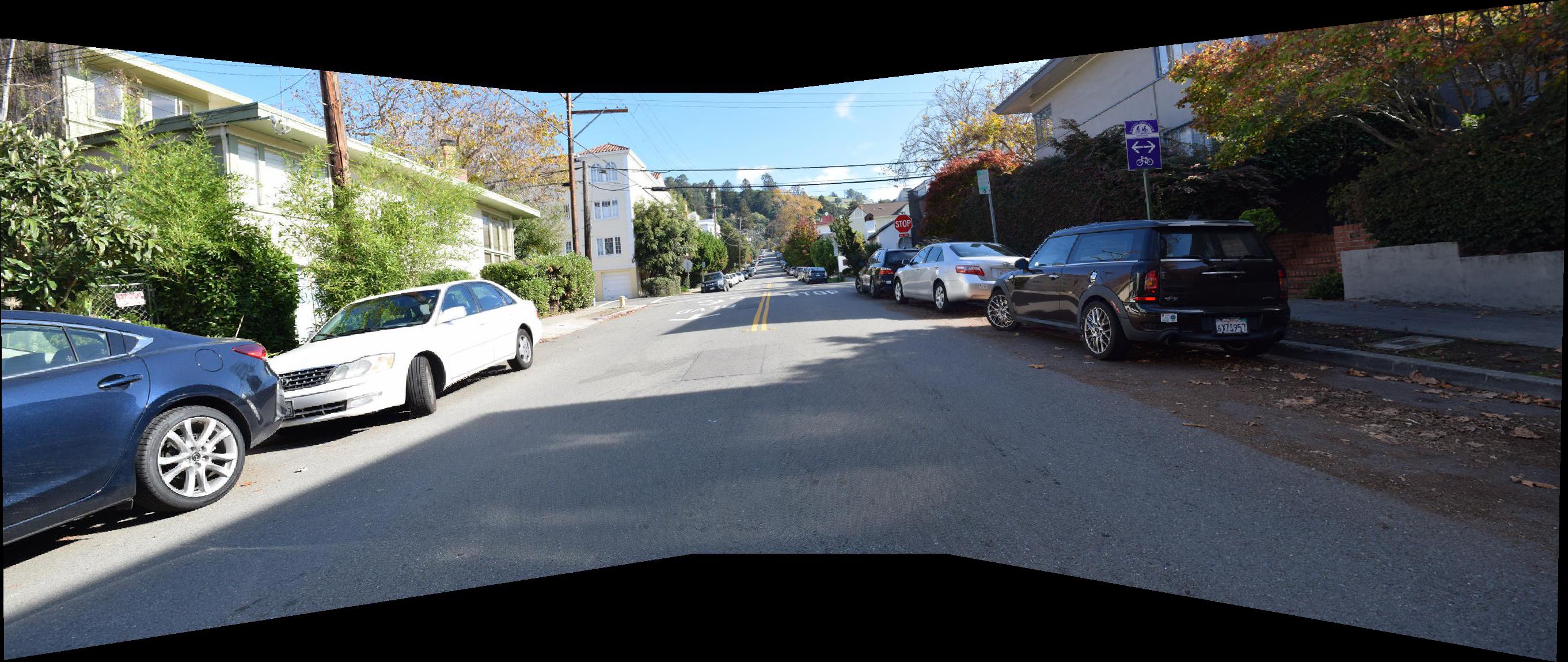
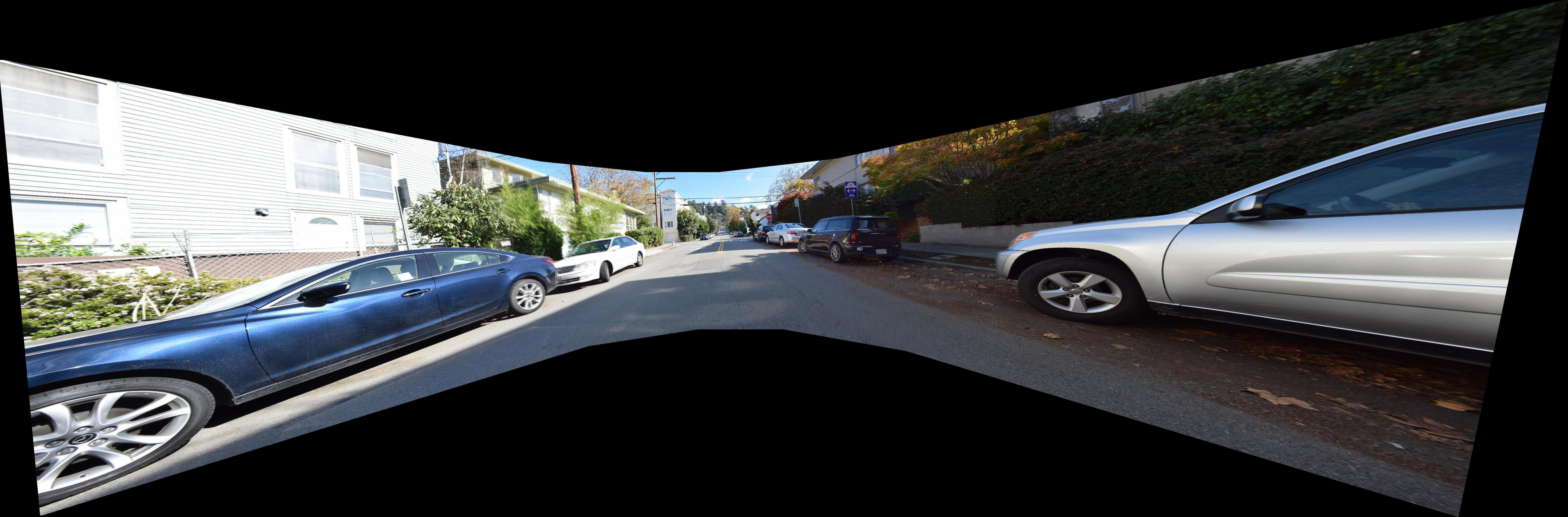
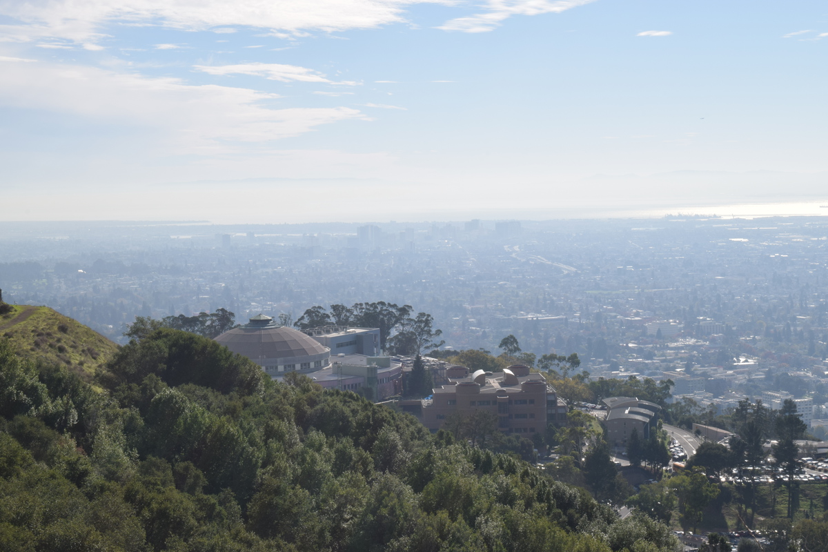
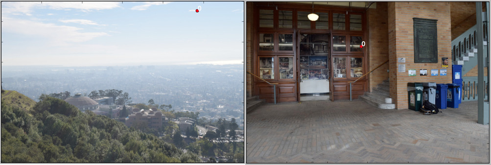
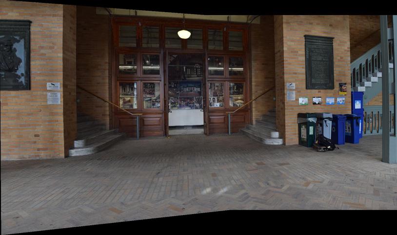
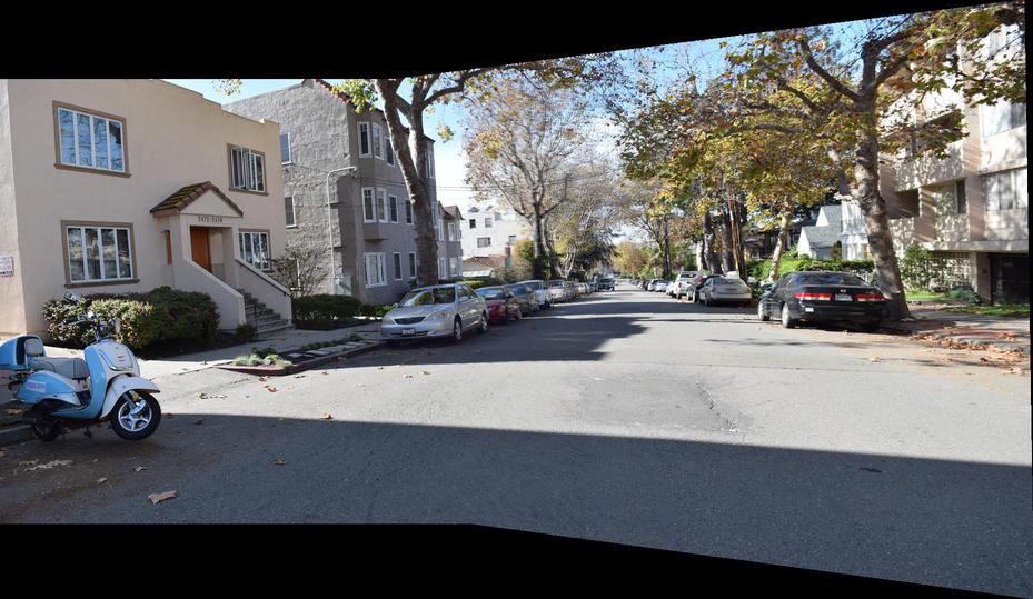
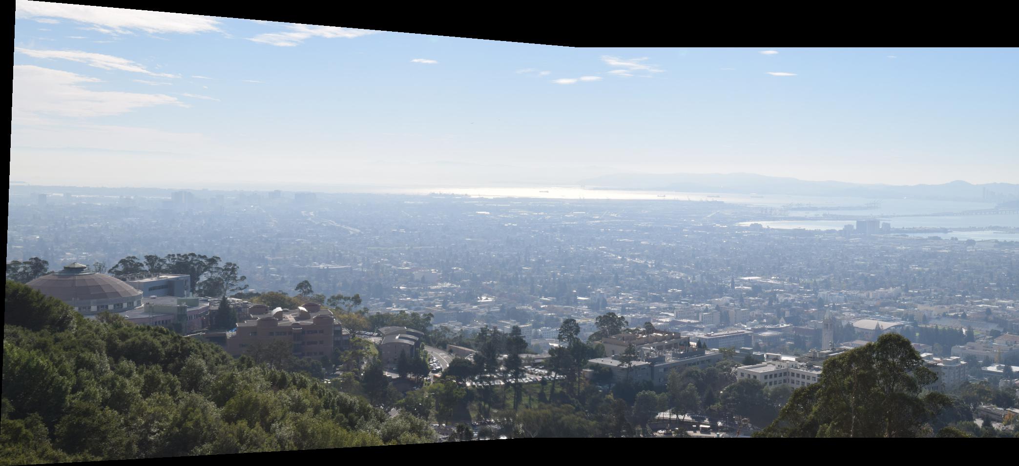
Below are some of my full panorama results:

Original Images

Warped Images with Center Image Fixed

A Beautiful View of the Bay from Lawrence Hall of Sciences

Original Images

Warped Images with Center Image Fixed

Inside of Hearst Memorial Mining Building

Original Images

Warped Images with Center Image Fixed

A View Down My Street (Middle 3 Images Used)

A View Down My Street (All 5 Images Used)

Original Images

Warped Images with Center Image Fixed

A View Up My Street (Middle 3 Images Used)

A View Up My Street (All 5 Images Used)

Results seem to vary depending on subject and the steadiness with which the photographer takes the pictures (since any non-lateral rotation of the camera can make the output image blurry). Additionally, the feature point selection greatly impacts the transformation. The pictures of the bay seem to turn out the best probably because of the high amount of entropy and loss of detail as the details of the scene are mostly small.

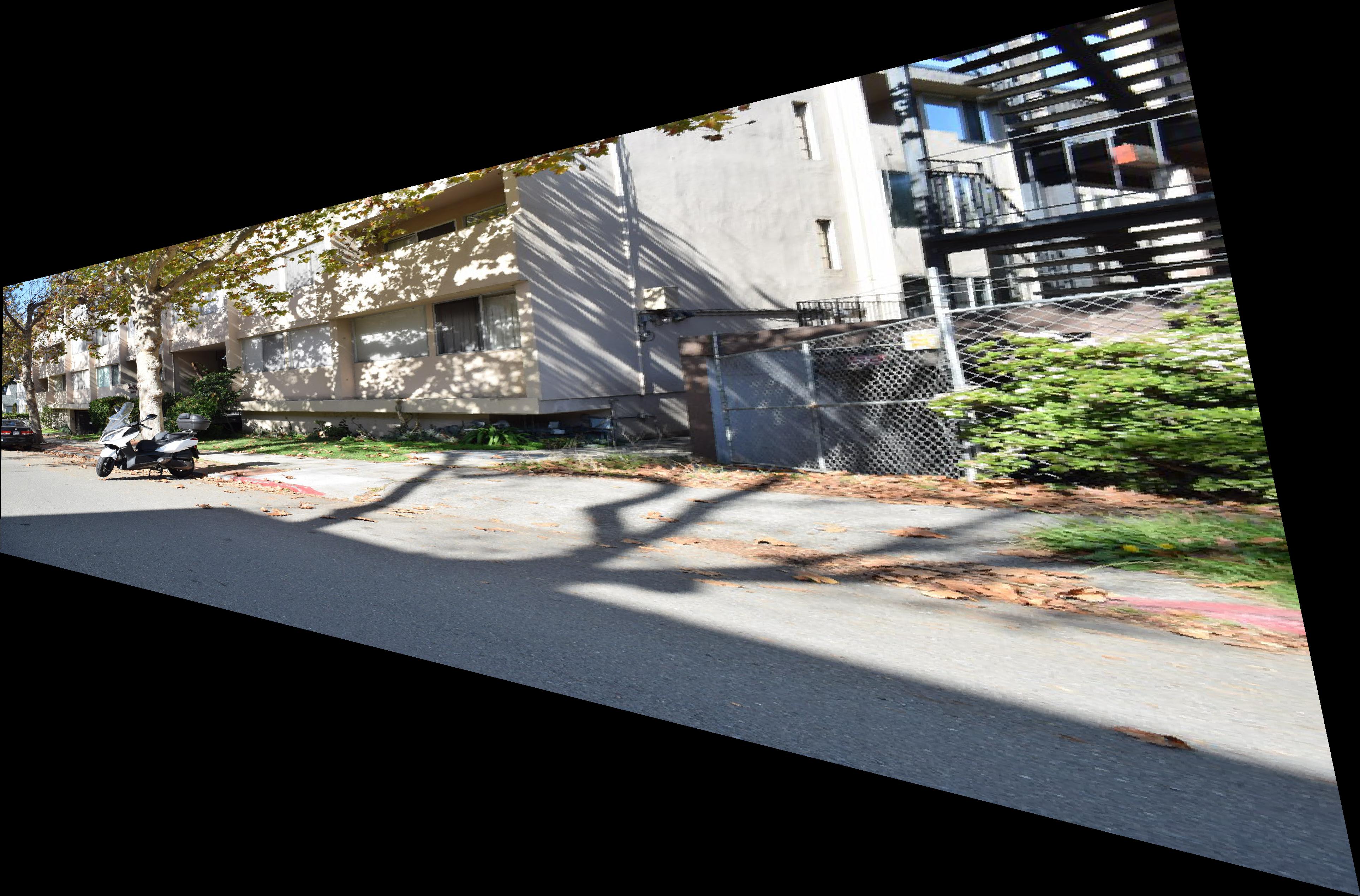
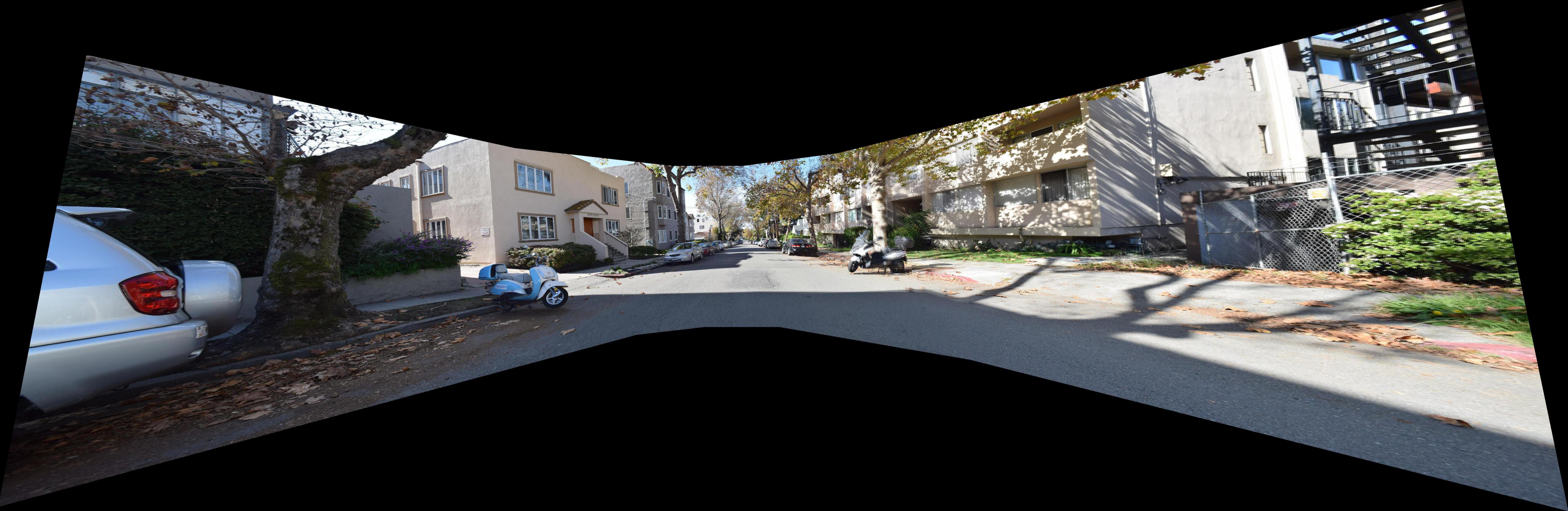
Interestingly, in the final 2 results where I used 5 panels rather than 3, it seems that the images on the far left and right warp a lot more than the rest of the images. This could again be the fault of the photographer as I took them with the camera at an upwards angle and thus as I rotated the camera, more of the scene changed. This is why the furthest right and left panels are so stretched out.

In part 2, I manually selected the feature points I wanted to use in the source images. However this is incredibly painstaking. The next parts of the project involve my implementation of auto-detection of feature points.

The first step in the overall feature detection algorithm is detecting potential feature points. In the previous part, we manually clicked and chose matching features in both images. We can distinguish potential feature points automatically by identifying corners in both images. A good method of doing so is via Harris corner detection which relies on computing a corner response map for the image, identifying regions with high responses, and finally taking only points of local maxima in relation to response. We also keep track of the response values for each of these points for use in the next part.

Below are some examples of my corner detection on the interior of Hearst Memorial Mining Building:

Original Left Panel (Warped)

Original Center Panel (Static)

Detected Harris Corners of Left Panel

Detected Harris Corners of Center Panel

As you can see, there are a large amount of harris corners which are detected within this 1200 x 800. I averaged around 22,000 detected corners for images of similar size.

Next, we apply adaptive non-maximal suppression to reduce the number of total potential feature points to a desired amount. First, we calculate a radius value r for every point xi for a given image I such that:

Note that:
f(x) = Harris corner response value for x
I = image
xi = Harris corner in I
xj = all other Harris corners in I

The c value designates when a neighboring corner xj will suppress the target corner xi. I used a c value of 0.9 so because c is large, we can safely assume that a neighbor xj will only suppress the current point xi if it is significantly stronger than xi. We now have a list of radii for each point xi such that the radius r is the radius in which xi is a local maxima. We then sort the radii values in descending order and take the first 500 entries (the 500 entries with the largest values of r) as our potential feature points. This guarantees that our chosen 500 feature points will be spread out to allow for the best chance at a good homography matrix. This is done separately for each image.

Below are the feature points from the previous part reduced to the 500 points with the highest values r in each image:

Left Feature Points after Adaptive Non-Maximal Suppression

Center Feature Points after Adaptive Non-Maximal Suppression

Next, we perform feature matching. We can define the feature descriptor of every point as the 8 x 8 patch of pixels centered at the point. However, naively taking this patch of pixels leaves our feature matcher susceptible to error due to differences in brightness and bias. In order to address these issues, we first take the 40 x 40 patch of pixels centered at the point and gaussian blur the patch (I used a sigma value of 1).

Then we downscale the image by a factor of 5 to get the 8 x 8 patch. Finally, we calculate the mean (mu) and standard deviation (std) of the descriptor and perform the following operation:

I' = (I - mu) / std

Now we have a set of feature descriptors and we can match features based on this. We take every feature descriptor in the image we want to warp and find the feature descriptor in the static image with the smallest SSD (call the SSD with the matched feature descriptor 1-NN). We also find the second best match (call this SSD 2-NN). Finally, call the pair of features (the feature descriptor in the image we want to warp and 1-NN) a match if and only if:

(1-NN) / (2-NN) < e

I used an e value of 0.3. We do this to rule out features that do not match well. In other words, we only keep the match if the best match SSD is much better than the next best match SSD, which makes the ratio between the two small. After doing this, we can see our remaining feature-matched points below:

Left Feature Points after Adaptive Non-Maximal Suppression

Center Feature Points after Adaptive Non-Maximal Suppression

Note that we could also flip the orientation to take feature descriptors of the static image and match them to the descriptors of the image we wish to warp. It does not matter as long as you end up with a list of pairings.

The final step in generating our homography matrix H is to use the random sampling consensus algorithm (RANSAC). RANSAC operates as a random algorithm whereby we randomly select 4 pairs of feature points and construct our homography matrix H as in the previous part of the project. This way, our H matrix tells us how to transform the points in the original image we wish to warp to the shape of the static image.

Once we have this matrix H, we transform all the other matched feature points of the image we wish to warp via H and check to see how close they are to their matched feature point counterparts. We score each homography H based on whether the SSD between the transformed point and matched feature point is lower than a given value e. I used e = 0.3.

We repeat this cycle for a large number of iterations (I chose to use 5000 iterations) and then take the highest scoring homography matrix and use it for the output image's warp. An example of the 4 pairs of feature points contributing to the best homography matrix is below:

Left Feature Points after RANSAC

Center Feature Points after RANSAC

Since the feature points are selected randomly, it possible to get different feature points used to construct the homography matrix across multiple runs of the algorithm. Below are some of my results from automatic homography generation as well as comparisons to my results from the previous part of the project:

Original Images

Warped Images with Center Image Fixed

Automatic: A Beautiful View of the Bay from Lawrence Hall of Sciences

Manual: A Beautiful View of the Bay from Lawrence Hall of Sciences

Original Images

Warped Images with Center Image Fixed

Automatic: Inside of Hearst Memorial Mining Building

Manual: Inside of Hearst Memorial Mining Building

Original Images

Warped Images with Center Image Fixed

Automatic: A View Down My Street (Middle 3 Images Used)

Manual: A View Down My Street (Middle 3 Images Used)

Automatic: A View Down My Street (All 5 Images Used)

Manual: A View Down My Street (All 5 Images Used)

Original Images

Warped Images with Center Image Fixed

Automatic: A View Up My Street (Middle 3 Images Used)

Manual: A View Up My Street (Middle 3 Images Used)

Automatic: A View Up My Street (All 5 Images Used)

Manual: A View Up My Street (All 5 Images Used)

As you can see in many cases the differences are difficult to tell. Since my results from the first part were fairly good, this suggests that the automatic homography generation was successful in general. In the 5 panel panoramas, however, the automatic algorithm seems to be slightly less successful especially in the "A View Down My Street" panorama where you can see the bike on the right side is more blurry in the automatic version than in the manual version.

Another thing to note is that knowing the correct orientation of the images, I chose to only sample Harris corners from a section on the left or right side of the image I chose to keep stationery. This section had height matching the static image but a width only as wide as the image we want to warp. This is because I set up my code to only combine two images at a time. So in order to construct 5 panel panoramas, the result of the first run of the algorithm is used as the stationery image in the next run of the algorithm.

Eventually, the input static image gets very large since it is a panorama in progress and so many Harris corners are detected however we only care about the ones near the edges of the panorama in progress. Thus we can save runtime and potential for error, as I did have problems adding my 5th image to my 5 panel panoramas when all Harris corners were being detected in the 4 panel input panorama.

For this project, we were tasked with implementing one final component called a bells and whistles feature. This feature was chosen by the student and was typically built on top of the required algorithm (in this project, this would be parts 1 - 6). For my bells and whistles portion of the project I decided to do panorama recognition. Given a set of unordered images, determine which images form panoramas and stitch them together. For this part of the project, we were instructed not to worry about bundle adjustment and only focus on pairwise homography estimation. The algorithm that I used was fairly simple:

1

2

3

4

5

6

An Example of an Input Image Set
Pairs should be: [1,5] and [3,4]

First, compute the harris points for all images in the input batch. Run adaptive non-maximal suppression on the points and then gather the feature descriptors for each image based on the resulting 500 feature points.

Next run a O(n^2) search for all matching pairs of images based on the number of RANSAC and feature matches. For every pair of images, the matching features are computed. Below are examples of pairs of images labeled with their matched features (any pairs without at least 1 pair of matched features was omitted):

[1, 4] after Feature Matching

[1, 5] after Feature Matching

[2,5] after Feature Matching

[3, 4] after Feature Matching

[3, 5] after Feature Matching

[4, 5] after Feature Matching

Then RANSAC is run over the matching features and the number of transformed feature points which are sufficiently close to their corresponding partner in the matching feature pairs is used as a score. The corresponding homography matrix H is also saved. In both RANSAC and feature matching, an e value of 0.3 is used to rule out any non-matches. Additionally, two images are considered to form a panorama only if they have a RANSAC score of 20 or more. Below are the matches with the points labeled that were used for the homography matrix:

[1, 5] with Feature Pairs used in Homography after RANSAC

[3, 4] with Feature Pairs used in Homography after RANSAC

Finally, take each image and find its best match based on the scores we just computed. Then proceed as before by taking the corresponding homography matrix to warp one image into the shape of the other. Then blend the images together and we are done. We arbitrarily set the image that we import first in the pair as the image we warp and the second as the image we set as static. Below are the results of the algorithm with the non-panorama images being ignored:

[1, 5] Warped, Aligned, and Blended

[3, 4] Warped, Aligned, and Blended

One limitation of this algorithm is that it can only match pairs of images. It will not be able to string together 3 images into the same panorama unless it is run multiple times and it won't be able to distinguish whether a given image is a center panel or not. Obviously you wouldn't be able to distinguish a center panel given a pair of images anyways but I imagine, in order to improve the algorithm, one could do the same feature matching but then see if multiple images met the RANSAC score threshold for a given image. Then, the average matched feature point for each matched image could be computed and compared. This mean feature point could then potentially be used to figure out the orientation of the images. If I had more time, this is the direction I would take to improve my algorithm.

Conclusion: What I Learned

This project taught me the importance of selecting good feature points and the gruelling process of correcting feature point errors. However, I enjoyed seeing the results of the blending technique I applied and the final product was extremely worthwhile.

The individual parts of the algorithm we implemented in this project are not particularly complex. However, it's very interesting to me to be able to see many of the simpler concepts we learned early on in the class coming together to form a comprehensive and highly effective algorithm.