Ray Tracer
CS 184 Project by David Hahn
Introduction
In this project, I implemented a ray tracer with global illumination, light sampling for diffuse objects, and adaptive sampling. This allowed me to render scenes with triangle meshes and spheres as well as simulate lighting on these meshes. the code that I wrote in the first part of project 3 and implemented reflective, refractive, and microfacet surfaces. Additionally, I also implemented environment lighting and depth of field which, overall, allows for more interesting renders.
Please note that during the class, this project was split up into two separate parts (first implementing the ray tracer and secod extending it to allow various non-diffuse material types amongst other features).
Finally, you'll notice that there are rendering options labeled beneath most of the images. The breakdown of the values is as follows:
- t: number of threads used
- s: pixel sampling rate (samples / pixel)
- l: light sampling rate (samples / light)
- m: maximum ray depth for indirect illumination
- alpha: roughness measure for microfacet material
- b: simulated ideal thin lens aperture
- d: simulated ideal thin lens focal length
Table of Contents
-
Ray Generation, Scene Intersection
-
Bounding Volume Hierarchy
-
Direct Illumination
-
Indirect Illumination
-
Adaptive Sampling
-
Mirror and Glass Materials
-
Microfacet Material
-
Environment Light
-
Depth of Field
Ray Generation and Scene Intersection
General Loop Procedure and Camera Ray Generation
The bread and butter of the ray tracer is the ray generation and sampling portion of the code. We begin by checking to see what sampling rate per-pixel has been requested. Then we loop for every sample we want to take and add a random value between 0 and 1 to the x and y of the pixel we want to sample. If the sampling rate is 1 sample per pixel, we simply use the center of the pixel for which we ad 0.5 to x and y.
In order to sample a pixel, we generate a ray with origin at the camera's position and a direction pointed from the camera to the pixel's world coordinates. To get the pixel's world coordinates, we first calculate the direction vector in terms of the camera's coordinate space which involves using the two given point of view angles. These angles map to the bottom left and top right corners of a sensor plane 1 unit along the view direction of the camera. We then map the pixel's x and y and translate and scale such that (0, 0) maps to the bottom left corner and (1, 1) maps to the top right.
Triangle and Sphere Intersection
However simply generating the rays is not enough to render a scene. In order to render, we need to detect the order by which objects in a given scene are intersected. To detect an intersection, I implemented the Moller Trumbore algorithm which relies on Cramer's rule in order to not only detect but also pinpoint the location of an intersection between a ray and a triangle. Cramer's rule gives us a solution in determinants for a given system of equations and Moller Trumbore uses the rule by setting up a system of equations to calculate $t$, the intersection value, and $b_1$ and $b_2$, barycentric coordinates $\beta$ and $\gamma$ respectively. The ray's direction and the triangle's verticles are used to construct the system of equations.
Finally, the last step of the intersection routine is to sanity check the values we receive. An intersection is only detected if $t$ is positive and $b_1$ and $b_2$ are between 0 and 1. Additionally, we only care about $t$ values within the bounds of the ray which are determined by the ray's $t_{min}$ and $t_{max}$ attributes. If we determine an intersection has occurred, we first update the ray's $t_{max}$ to the detected $t$ value. This is so that future samples of the same ray against other triangles do not consider any objects as intersected unless they are closer than the closest object encountered thus far. Then, we can either return true and are finished or we update the given intersection struct to hold:
- the $t$ value of the intersection
- the BSDF of the triangle (relevant later)
- the normal (which we calculate by interpolating $(1 - b_1 - b_2)$, $b_1$, and $b_2$ with the triangle normals)
- and the intersected primitive which is a reference to the triangle we have tested
I additionally implemented sphere intersection which involves calculating an $a$, $b$, and $c$ value dependent on the ray's origin and direction and the sphere's origin and radius and using the quadratic formula to determine the number of intersections as well as the location of the intersection(s) if they exist. Similar bounds checking with the ray's $t_{min}$ and $t_{max}$ were done here as well.
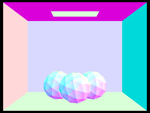
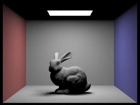
Below are my results on some small scenes (the objects' color is dependent on the surface normal at the intersection point). The scene of the spheres has 14 primitives while the scene with gems has 252. Scenes with more primitives than these took considerably longer to render. For example, the teapot mesh took 100 seconds while the gems took 10 seconds and the spheres took less than 1 second. The runtimes seem to scale linearly (at least for these smaller jobs). Larger meshes, like the Max Planck mesh, which has 50,000 primitives, were too slow to render in a reasonable amount of time.
CBspheres_lambertian.dae
14 primitives
[t, 8] [s, 1] [l, 1] [m, 0]
teapot.dae
2464 primitives
[t, 8] [s, 1] [l, 1] [m, 0]
CBgems.dae
252 primitives
[t, 8] [s, 1] [l, 1] [m, 0]
Without proper illumination calculations in place, the colors of the surfaces are simply determined by the angle of the surface normal. Additionally, any images prefixed with "CB" indicate that the model is enclosed within a model of a Cornell Box.
Bounding Volume Hierarchy (BVH)
BVH Construction
In this part, I implemented bounding volume hierarchies. These are binary trees which allow us to detect intersections more quickly by traversing the tree structure rather than testing against all primitives naively. To begin, we must construct the BVH. The skeleton code gave me a node struct with left and right members as well as a bounding box attribute. Then, if the number of primitives we need to store is less than the max number of primitives allowed on a leaf node, we calculate the bounding box of the node and store the primitives and we are done.
Otherwise, we compute the bounding box as well as a centroid box (which is a bounding box expanded using the centroids of each primitive). We then take the largest axis of the extent of the bounding box and use this as the axis to split on. If a given primitive's centroid value on this axis is smaller than the centroid box's centroid value on the axis, we place the primitive in a list to be evaluated on the left child of the current node. If it is larger, we place the primitive in a list to be evaluated on the right child. We then recursively call the construct method on these primitives lists.
We split using the centroid box's centroid rather than the bounding box's centroid because the bounding box's centroid is not guaranteed to split the primitives whereas the centroid box's centroid is as long as the centroids of the primitives are not all the same. In the case they are, I have an additional catch-all section of code which splits the primitives arbitrarily in half by the order in which they are ordered in the input list.
BVH Intersection and Acceleration
Now that we have our BVH data structure, we can check intersections with the individual nodes. Each node has a bounding box which we've pre-computed. In order to check whether we intersect that bounding box, we compute the t location where the ray touches the min and max corners of the box in the x, y, and z axes. We then compare these t values against each other to determine whether an intersection has occurred. For each axes, we compute 2 values since we compare the ray against two corners of the box. This gets us: $$tx_1, tx_2, ty_1, ty_2, tz_1, tz_2$$ We can then compute the following values: $$min_x = min(tx_1, tx_2)$$ $$max_x = max(tx_1, tx_2)$$ $$min_y = min(ty_1, ty_2)$$ $$max_y = max(ty_1, ty_2)$$ $$min_z = min(tz_1, tz_2)$$ $$max_z = max(tz_1, tz_2)$$
First, we compare the x's to see if they exceed the bounds of the y's. So we check tx_min to see if it is greater than ty_max. Likewise we check if tx_max is smaller than ty_min. If either of these are true, we know that an intersection cannot occur because the ray enters one axes after exiting the other or exits one axes before entering the other.
Then, we take max(tx_min, ty_min) and min(tx_max, ty_max) and compare against the computed min and max tz values similarly. If neither of the aforementioned cases is true, we detect an intersection. We determine: $$t_{min} = max(t_z, max(min_x, min_y))$$ $$t_{max} = min(t_z, min(max_x, max_y))$$ and simply check to see if the intersection occurs within the valid bounds of the ray (using the ray's $t_{min}$ and $t_{max}$) to make a final decision on the detection. Additionally, we take the min of the maxes and the max of the mins because we want to check the innermost value for the intersection since a ray could travel further than the absolute min of the mins and then intersect the secondary axis later on, given the correct direction and origin and location of the bounding box.
Now that we can detect intersections of the bounding box, we can run through our BVH intersection detection. Any given node in the BVH has a bounding box so we check to see if the ray intersect the bounding box. If it does not, we are done and we return false back. If it does, we need to check whether the node is a leaf. If it is, we check all the primitives contained at the leaf node. All the updating of the ray's $t_{max}$ and the intersection object should be done in the primitives' intersect methods so we don't need to worry about that. Additionally, if the node is not a leaf, we recursively descend to both children and check for intersections there.
This method allowed me to render scenes and meshes with much larger amounts of primitives. Below are a few examples:
maxplanck.dae
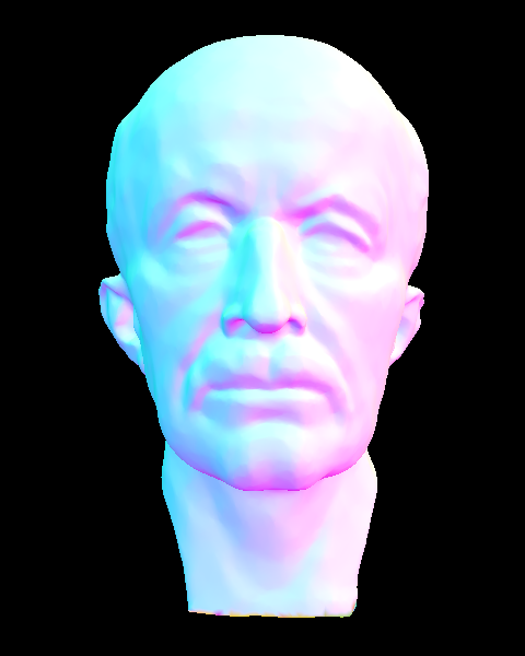
50801 primitives
[t, 8] [s, 1] [l, 1] [m, 0]
beast.dae
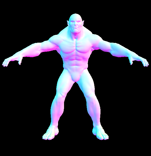
64618 primitives
[t, 8] [s, 1] [l, 1] [m, 0]
peter.dae
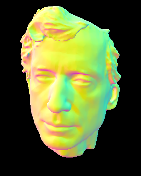
40018 primitives
[t, 8] [s, 1] [l, 1] [m, 0]
As mentioned before, without proper illumination calculations in place, the colors of the surfaces are simply determined by the angle of the surface normal. Here are some more renders done with dae files using Cornell Boxes.
CBlucy.dae
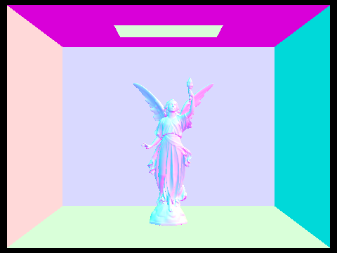
133796 primitives
[t, 8] [s, 1] [l, 1] [m, 0]
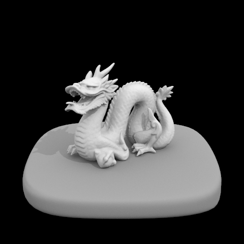
CBdragon.dae
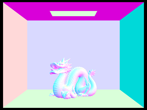
100012 primitives
[t, 8] [s, 1] [l, 1] [m, 0]
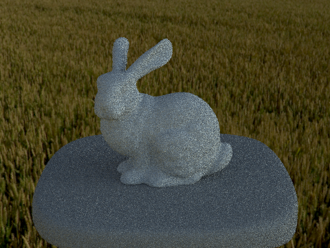
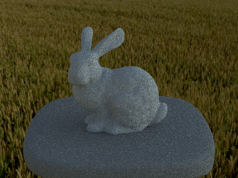
CBbunny.dae
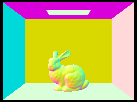
28588 primitives
[t, 8] [s, 1] [l, 1] [m, 0]
Direct Illumination
Diffuse BSDF Material
In this part of the project, I implemented BSDF reflectance sampling for diffuse materials and an algorithm for estimating the amount of light directly hitting an object. The sampling was fairly straightforward. Because a diffuse material scatters light in a hemisphere around the hit point equally, we simply use the BSDF object's reflectance and return it. We divide by $\pi$ before returning it because the integral over a hemisphere of a cosine is $\pi$.
Direct Lighting Calculation
The estimation algorithm we use involves an approximation of the integral of the product of the light's radiance, the object's reflectance, and a cosine product which, according to Lambert's law, is the dot product between the normal vector to the surface and the ray representing the incoming light ray. Because we want this estimation to be at most 1, we need to scale the reflectance by $\pi$.
The rest of the estimation algorithm is as follows. For any given intersection with a primitive in the scene:
- Iterate over each light
- Iterate over the number of samples per light (which is set by the -l command line flag argument)
- If the light is a delta light, only take 1 sample since all samples will be identical
- Sample the incoming radiance of the light and save the probability with which this point of light was sampled for the later calculation.
- Check if the sampled point of the light is behind the object. If it is, continue.
- Create a shadow ray from the hit point in the direction of the sampled light point and check to see if it intersections the BVH anywhere.
- If it does, continue sampling. This indicates the shadow ray hit another object before getting to the light.
- If it does not, calculate the value of the product of the light's incoming radiance, the refletance of the object, and the cosine term. Divide by the probability with which this sample was chosen to normalize across individual samples.
- Sum these calculated values.
- Take the sum of the values for the given light and divide by the number of samples to normalize across lights.
- Add this normalized sum to the overall accumulation representing the amount of light hitting the surface at the given point.
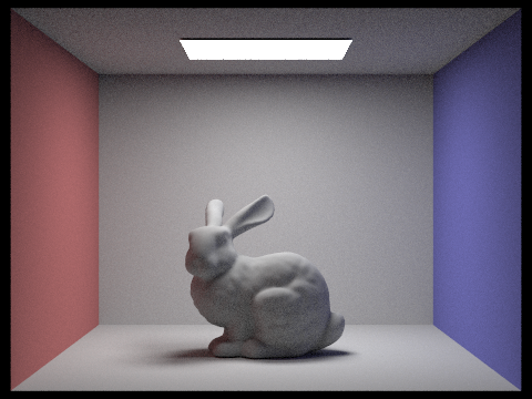
After doing this, scenes with diffuse objects are render-able with direct lighting. Here are a couple examples:
CBspheres_lambertian.dae
[t, 8] [s, 64] [l, 32] [m, 0]
dragon.dae
[t, 8] [s, 64] [l, 32] [m, 0]
CBbunny.dae
[t, 8] [s, 64] [l, 32] [m, 0]
As you can see, the dragon looks fairly realistic but the other scenes are a little less-so. This is because our eyes are trained to distinguish realism and the light in the CB_____.dae files are boxes enclosing objects where our brains expect light to bounce off the walls of the box and interact with objects in that manner. That part of the lighting estimation is implemented in indirect illumination, the next part.
Additionally, this method is prone to noise at low sampling rates for lights. The following images are for the bunny scene where I fixed the sampling rate at 1 and changed the number of samples I took per light. This occurs because a low per-light sampling rate may cause shadow rays which intersect with objects other than the light more likely so a single faulty sample will have more governance on the overall quality of the image.
Lowest samples per light
(CBbunny.dae)
[t, 8] [s, 1] [l, 1] [m, 0]
(CBbunny.dae)

[t, 8] [s, 1] [l, 4] [m, 0]
(CBbunny.dae)

[t, 8] [s, 1] [l, 16] [m, 0]
Highest samples per light
(CBbunny.dae)
[t, 8] [s, 1] [l, 64] [m, 0]
Indirect Illumination
Indirect Lighting Calculation
I then implemented indirect illumination using an algorithm to approximate the light bouncing off other objects and landing on a given surface. The algorithm is as follows:
- Generate all camera rays with max_depth set to the argument following the -m flag. This determines the maximum number of bounces we check for light.
- Sample the BSDF such that you receive an incoming light ray and corresponding probability.
- Take the sampled reflectance and take the illuminance of that, which should be between 0 and 1.
- I scaled the illuminance by 10 and added 0.05 to it so that it wouldn't be too low, causing the algorithm to terminate early.
- Take the illuminance value and use it in a coin flip as the probability of continuing (a low illuminance value should result in a lower chance of continuing).
- If we terminate, return a 0-spectrum.
- If we continue, use the sampled incoming light ray and recursively run the trace_ray procedure on it.
- Take the incoming radiance returned by the trace_ray and multiply by the cosine term (defined above) and the sampled BSDF reflectance. Additionally, divide by the probability of the sampled incoming light ray as well as (1 - probability of continuing).
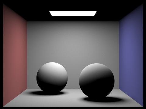
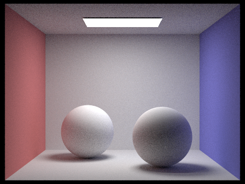
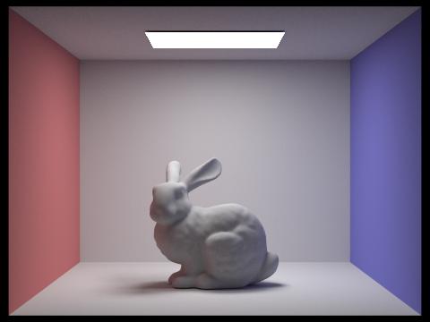
Once this part of the project is completed, many of the CB scenes are more realistic when rendered, especially the spheres. Below are some of my results (with direct lighting only, indirect lighting only, and both):
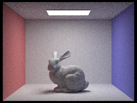
Direct Illumination Only
(CBspheres_lambertian.dae)
[t, 8] [s, 64] [l, 32] [m, 0]
Global Illumination
(CBspheres_lambertian.dae)
[t, 8] [s, 64] [l, 32] [m, 5]
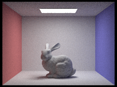
Indirect Illumination Only
(CBspheres_lambertian.dae)
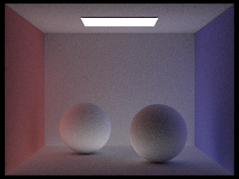
[t, 8] [s, 64] [l, 32] [m, 5]
Below are renders of the bunny scene with fixed per-pixel and per-light sampling rates but varied maximum ray depths (which is set by the -m command line argument). As you can see, a max depth of 0 is the same as direct lighting only and the influence of indirect lighting increases slightly as the algorithm is allowed to traverse more hops (after the first hop of course). However, eventually we hit a point where increasing the maximum depth does not really alter the image by much (compare the depth 5 and depth 100 images). I imagine that maximum ray depth will have more impact if a larger scene is rendered with more lights and more objects.
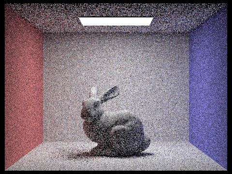
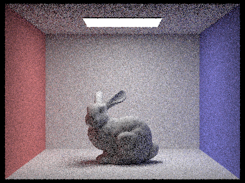
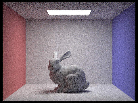
Lowest Indirect Ray Depth
(CBbunny.dae)
[t, 8] [s, 64] [l, 32] [m, 0]
(CBbunny.dae)
[t, 8] [s, 64] [l, 32] [m, 1]
(CBbunny.dae)

[t, 8] [s, 64] [l, 32] [m, 2]
(CBbunny.dae)

[t, 8] [s, 64] [l, 32] [m, 3]
(CBbunny.dae)

[t, 8] [s, 64] [l, 32] [m, 5]
Highest Indirect Ray Depth
(CBbunny.dae)
[t, 8] [s, 64] [l, 32] [m, 100]
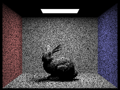
Additionally, here is the same scene with varied sampling rates and fixed maximum ray depth and per-light sampling rate. Again, sampling rate simply changes the amount of noise in the image due to per-pixel sampling. Adding in indirect illumination does not subvert the problem of a sampling rate being too low and introducing lots of noise.
Lowest samples per pixel
(CBbunny.dae)
[t, 8] [s, 1] [l, 4] [m, 5]
(CBbunny.dae)
[t, 8] [s, 2] [l, 4] [m, 5]
(CBbunny.dae)
[t, 8] [s, 4] [l, 4] [m, 5]
(CBbunny.dae)
[t, 8] [s, 8] [l, 4] [m, 5]
(CBbunny.dae)
[t, 8] [s, 16] [l, 4] [m, 5]
(CBbunny.dae)

[t, 8] [s, 64] [l, 4] [m, 5]
Highest samples per pixel
(CBbunny.dae)
[t, 8] [s, 1024] [l, 4] [m, 5]
Adaptive Sampling
Adaptive Algorithm
Finally, for all the previous parts, we've been sampling the entire per-pixel sampling rate number of samples. However if we use an adaptive sampling, it's possible to not calculate extra samples that may not change our overall pixel value by very much. Across multiple samples, we essentially attempt to calculate the point at which the samples so far have converged. Once this occurs, we deem it safe to exit out of the sampling routine and move onto the next pixel to be sampled.
In more detail, the procedure is as follows:
- Every time we calculate a sample $x_i$, add to values $s_1$ and $s_2$ such that (where $n$ is the number of samples taken so far): $$s_1 = \Sigma_{i=1}^{n} x_i$$ $$s_2 = \Sigma_{i=1}^{n} x_i^2$$
- Now, we calculate the mean and variance: $$\mu = \frac{s1}{n}$$ $$\sigma^2 = (\frac{1}{n - 1}) * (s2 - (\frac{s1^2}{n}))$$
- Once we've calculated the mean and variance, we can calculate the index of confidence I: $$I = 1.96 * \frac{\sigma}{\sqrt{n}}$$
- We multiply by 1.96 because this is the value for the confidence interval for 95% confidence. That is, we can be 95% confident that we've converged to a value within the given tolerance (defined below) by using the magic number 1.96.
- Finally, we test I against the product of the maxTolerance, which is user defined but set to 0.05 by default, and the mean:
- If $I <= maxTolerance * \mu$:
- We've converged with 95% confidence and can exit our sampling routine
- If $I > maxTolerance * \mu$:
- We haven't converged with 95% confidence and must continue sampling
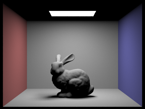
In utilizing this routine, we do not expect much difference in the output images. Given a reasonable tolerance level, the output images should not differ: only the sampling rate images should change. Here is a high quality render that I was able to complete reasonably quickly thanks to adaptive sampling.
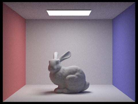
CBbunny.dae

[t, 8] [s, 2048] [l, 1] [m, 5]
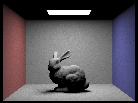
CBbunny.dae
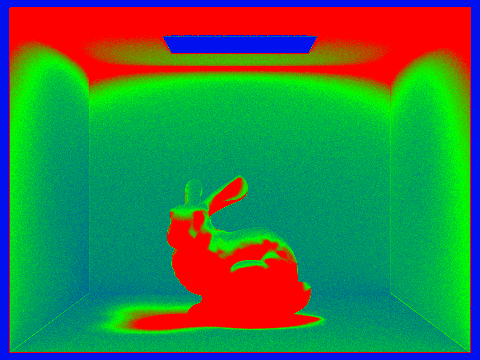
Adaptive sampling rate
The sampling rate image displays red for regions which are sampled thoroughly and blue for regions which are sampled sparsely. Green is used for everything in between. We can see that the underside of the bunny and the top panel of the box are sampled the most, most likely because they are deeply affected by indirect lighting for which samples may vary. On the other hand, the light at the top is not sampled very much and likewise with the regions outside the box. This is because the light and the regions outside the box are plain white and black respectively and do not require many samples to converge.
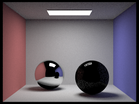
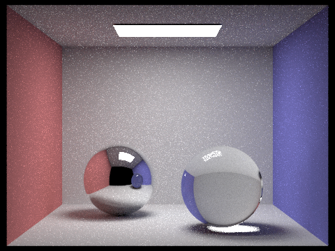
Mirror and Glass Materials
Reflection and Refraction
In order to implement mirror and glass materials, I had to write the functions for reflection and refraction of BRDF surfaces. In addition, I implemented probability-based sampling to simulate glass materials which have both reflective and refractive properties.
Reflection is fairly simple with the incoming ray to a surface just being reflected over the surface normal. Refraction is a little more tricky as we first need to check a ray and the material for total internal reflection (the case where the ray reflects back into the material). If not, then the incoming light rays follow the laws of physics with the angle of refraction following from Snell's law and the specifications in the project spec.
With the ray reflection function out of the way, perfectly reflective materials can be simulated simply by reflecting the input light ray over the surface normal of the object and calculating the irradiance with 0 fall-off. One extra consideration we need to consider is that the irradiance must be divided by the cosine of the angle formed by the outgoing light ray and the surface normal to counter the same term used in our indirect lighting estimate. This term usually serves the purpose of causing light fall-off but perfectly reflective materials lack this fall-off.
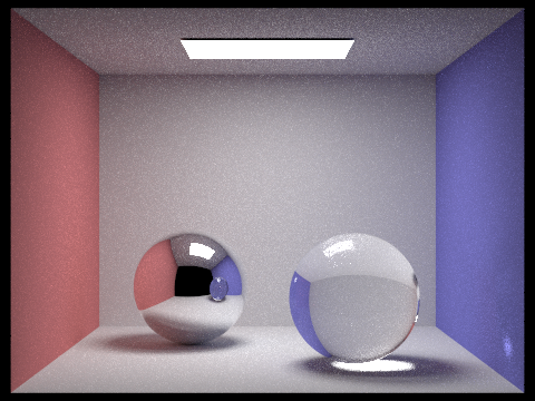
Glassy Material
However, glassy materials have both properties of reflection and refraction. In this case, we use a value called Schlick's approximation as a probability to sample between reflected and refracted rays. This is of course if total internal reflection of the ray does not occur. If the light is reflected, we calculate the irradiance at the given surface point by scaling the reflectance of the material by the probability with which we sampled reflection. If the light is refracted, we use another constant of the material called transmittance which designates how much light is transmitted through the material and scale by the probability with which we sampled refraction.
Other than that, there are some other constants we need to keep track of in our final irradiance calculation (for example we divide transmittance by the index of refraction value squared) to simulate the behavior of light, namely, the fact that radiance concentrates in light rays that enter materials with higher indices of refraction and less-so in materials with lower indices of refraction.
Here are some of my results:
CBlucy.dae
[t, 8] [s, 256] [l, 4] [m, 7]
Here is a series of images showing glass spheres in a Cornell box set at different max ray depths:
Lowest Indirect Ray Depth
(CBspheres.dae)
[t, 8] [s, 64] [l, 4] [m, 0]
(CBspheres.dae)
[t, 8] [s, 64] [l, 4] [m, 1]
(CBspheres.dae)
[t, 8] [s, 64] [l, 4] [m, 2]
(CBspheres.dae)
[t, 8] [s, 64] [l, 4] [m, 3]
(CBspheres.dae)
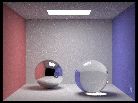
[t, 8] [s, 64] [l, 4] [m, 4]
(CBspheres.dae)

[t, 8] [s, 64] [l, 4] [m, 5]
Highest Indirect Ray Depth
(CBspheres.dae)

[t, 8] [s, 64] [l, 4] [m, 100]
Viewing these images, we can see that the spheres are not affected by direct lighting very much at all. In fact, most of their content is decided by the indirect lighting. As the number of maximum bounces increases, more and more detail is recovered in terms of the reflection and refraction of the indirect light rays. Additionally, after a certain point, adding more bounces does not make much of a visible difference for this resolution. This can be seen by comparing the max ray depth of 5 and 100 which look almost identical.
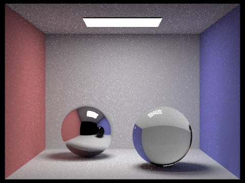
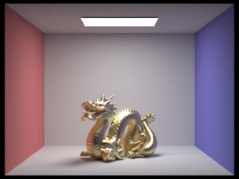
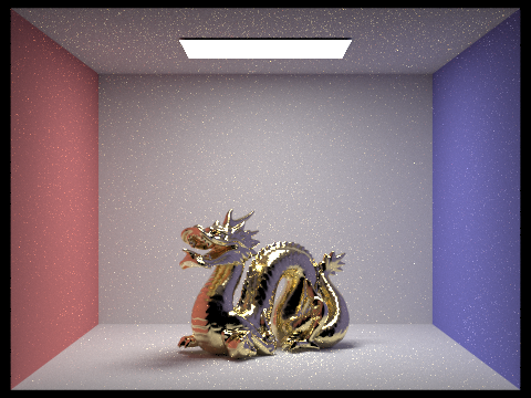
Microfacet Material
Microfacet BRDF
In this part, I implemented microfacet materials where materials have many small imperfections or textures, giving them a rough, brushed appearance. Because of this, we must importance sample light rays which bounce off this type of material since capturing every tiny facet of the rough material is incredibly data-inefficient. The details of the microfacet BRDF's irradiance calculation are captured in the project spec so I won't recite them here. At a high level, the surface irradiance of a microfacet material can be calculated via a Fresnel term, shadow-masking term, and a normal distribution function (in our case we used the Beckmann distribution). These values together estimate the irradiance of a rough material.
Importance Sampling
I additionally implemented importance sampling for microfacet materials. Importance sampling allows the renderer to converge more quickly (with less samples), giving improvements to rendering noise primarily with indirect lighting calculations.
Importance sampling for the microfacet surface primarily involves sampling a angle bisector vector given an incoming light ray which serves as the surface normal used in the NDF calculation. We begin by sampling two values [0, 1) that we then convert into a theta and phi value representing some given (angle bisector) half vector. Now that we have this vector, we can calculate the outgoing vector. However we also need to consider the probability distribution for this sample. The probability of choosing the theta and phi values can be calculated and then used to calculate the probability of sampling the half vector. Finally, we use this probability to calculate the probability of sampling the given outgoing light ray.
Again the specifics of the probability calculations are captured in the spec so I won't just recite them here. However the most significant idea is that the vector and its pdf are calculated via importance sampling rather than uniform sampling to emulate the roughness of the material.
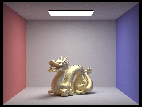
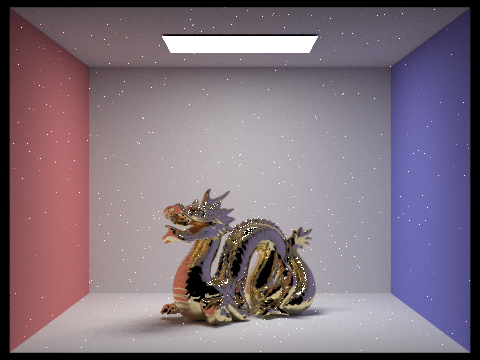
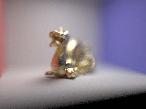
Below are some of my results for the gold microfacet dragon in the Cornell box with varied alpha values:
Highest alpha, most rough
(CBdragon_microfacet_au.dae)
[alpha, 0.5]
[t, 8] [s, 512] [l, 1] [m, 5]
CBdragon_microfacet_au.dae
[alpha, 0.25]
[t, 8] [s, 512] [l, 1] [m, 5]
CBdragon_microfacet_au.dae
[alpha, 0.05]
[t, 8] [s, 512] [l, 1] [m, 5]
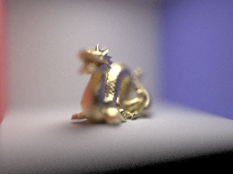
Lowest alpha, least rough
(CBdragon_microfacet_au.dae)
[alpha, 0.005]
[t, 8] [s, 512] [l, 1] [m, 5]
Varying the alpha value changes the roughness of the material with the higher alpha giving a more brushed look and a lower alpha giving a more reflective metal material look. Interestingly enough, noise increases when alpha is small.
Additionally, below are my results comparing uniform cosine hemisphere sampling to importance sampling:
Uniform Cosine Hemisphere Sampling
(CBbunny_microfacet_cu.dae0
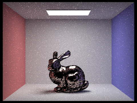
[t, 8] [s, 64] [l, 1] [m, 5]
Importance Sampling
(CBbunny_microfacet_cu.dae)
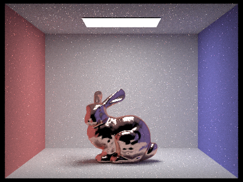
[t, 8] [s, 64] [l, 1] [m, 5]
Environment Light
2D to 3D Spherical Mapping
In this part of the project, I implemented environment lights. Essentially, we map a 2D texture to a 3D sphere (which our camera resides within) and then use the texture as a continuous source of light. In order to sample the environment light for radiance values, I had to construct a map representing the PDF function for a given texture. Below is the map I created for the field.exr file:
PDF Environment Map for field.exr
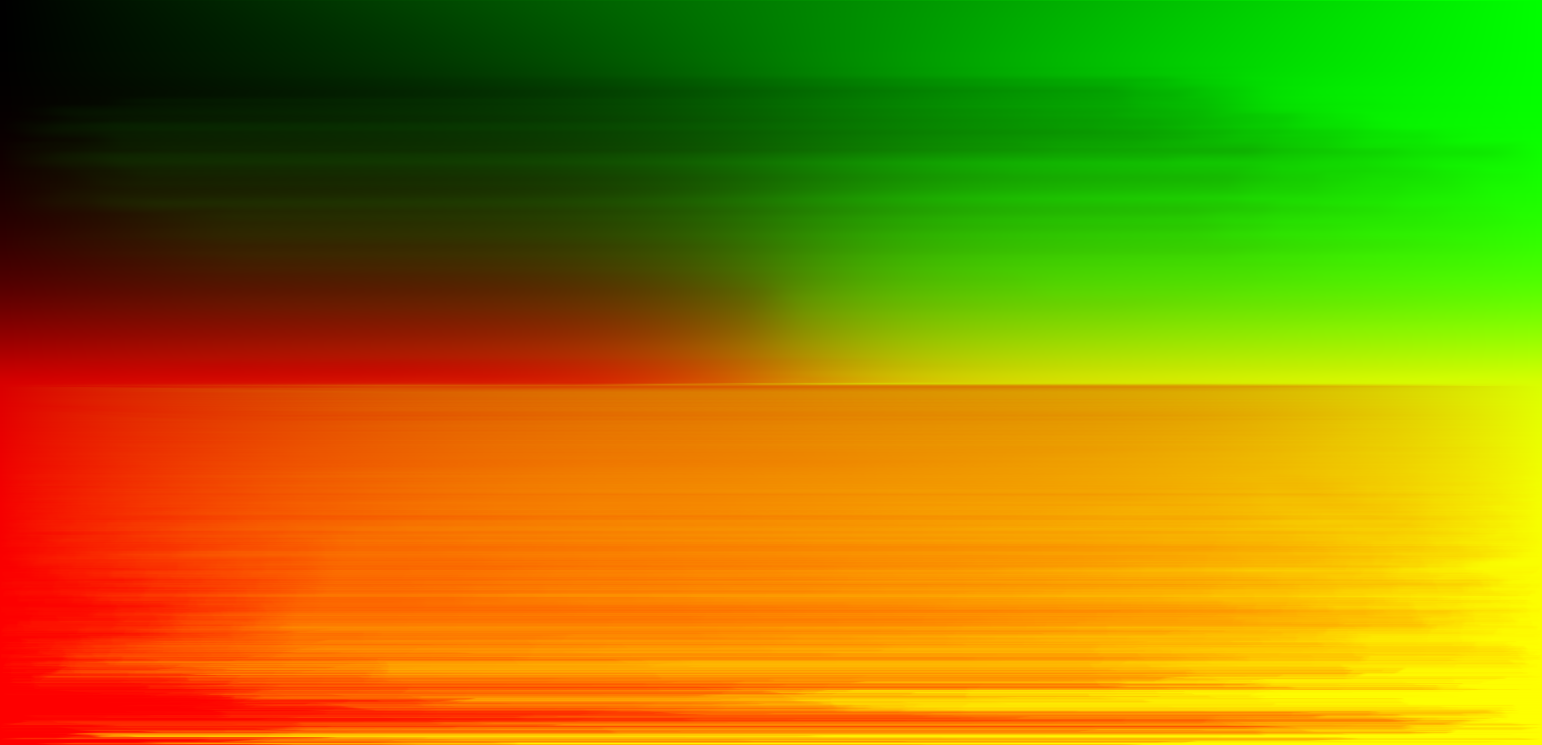
This part of the project required a little bit of intelligent algorithm design to avoid nested loops which tremendously slow down the PDF map generation. I was able to remove repetitive loops and pre-compute values to make the generation reasonably fast where the naive method was quite slow.
Next, I implemented the mapping of the environment light from the camera's perspective. This essentially takes a camera ray and converts to a spherical coordinate value and then converts this value to an XY value to sample on the 2D texture.
Importance Sampling
Finally, I implemented both uniform and importance sampling of the 2D texture as a light source. The former samples uniformly over the sphere whereas the latter samples from the PDF environment map I mentioned above. It takes advantage of some marginal and conditional probability maps we also set up in the above generation to perform the CDF inversion method to determine the pixel in the 2D texture to sample.
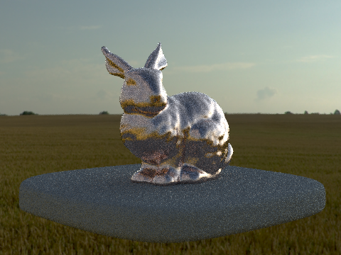
Below are some of my results comparing the copper microfacet bunny rendered in the field.exr environment light:
Uniform sampling
(bunny_microfacet_cu.dae)
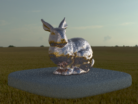
[t, 8] [s, 64] [l, 4] [m, 1]
[t, 8] [s, 4] [l, 64] [m, 5]
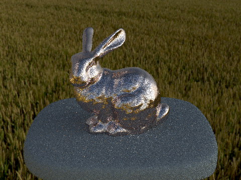
Importance sampling
(bunny_microfacet_cu.dae)
[t, 8] [s, 4] [l, 64] [m, 5]
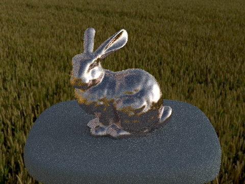
[t, 8] [s, 4] [l, 64] [m, 5]
With the microfacet bunny, there is a clear difference in the amount of noise between the uniform and importance sampling. At lower sampling rates, importance sampling converges much more quickly and we can see the difference above.
I additionally rendered the regular non-copper bunny with both sampling methods:
Uniform sampling
(bunny.dae)
[t, 8] [s, 4] [l, 64] [m, 5]
Importance sampling
(bunny.dae)
[t, 8] [s, 4] [l, 64] [m, 5]
The difference here is a very slight change in color. I suspect there is a lack of difference in terms of noise because of the reflective nature of the microfacet material being more prone to noise. I believe the white dots visible on the stand that the bunny sits on in the uniform sampling images for the microfacet bunny are caused by unrepresentative light rays bouncing off the bunny into the stand. However when the bunny itself is made of a diffuse material with higher light fall-off per bounce, this problem is less visible.
Depth of Field via Ideal Thin Lens Simulation
Focal Length Variance
Finally, I implemented an interesting depth of field algorithm to allow our renders to simulate a camera aperture using a perfect thin lens and subsequent depth of field effects. This procedure involved updating our camera ray generation process to make use of the refractive properties of the ideal thin lens.
Below are some of my results where I vary the focal length to focus on different parts of the dragon (the aperture value is designated by 'b' and the focal length is designated by 'd'):
Lowest focal length
(CBspheres_lambertian.dae)
[b, 0.25] [d, 2.1]
[t, 8] [s, 128] [l, 8] [m, 5]
(CBspheres_lambertian.dae)
[b, 0.25] [d, 2.3]
[t, 8] [s, 128] [l, 8] [m, 5]
(CBspheres_lambertian.dae)

[b, 0.25] [d, 2.5]
[t, 8] [s, 128] [l, 8] [m, 5]
Highest focal length
(CBspheres_lambertian.dae)
[[b, 0.25] [d, 2.7]
[t, 8] [s, 128] [l, 8] [m, 5]
As you can see as the focal length increases, parts of the scene that are further away come into focus. However because the aperture is fixed, the size of the area in focus (depth of field) does not substantially change.
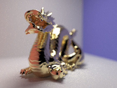
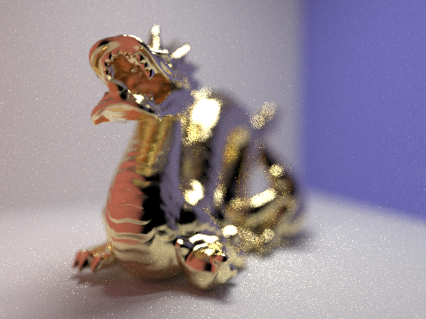
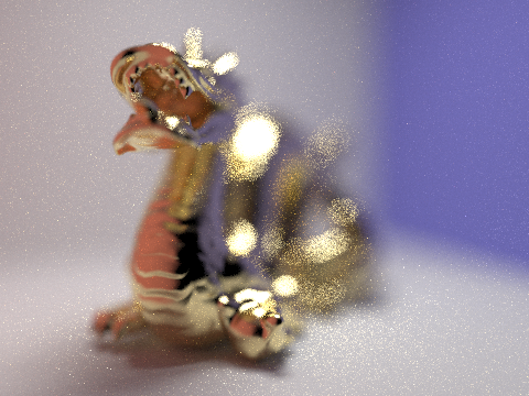
Aperture Variance
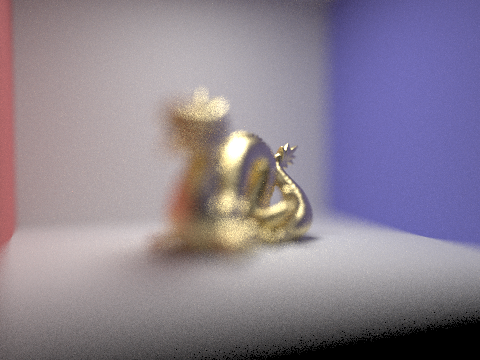
Below are renders of the same dragon except with different aperture values:
Smallest aperture
(CBdragon_microfacet_au.dae)
[b, 0.031250] [d, 1.1]
[t, 8] [s, 256] [l, 4] [m, 8]
(CBdragon_microfacet_au.dae)
[b, 0.044194] [d, 1.1]
[t, 8] [s, 256] [l, 4] [m, 8]
(CBdragon_microfacet_au.dae)

[b, 0.062500] [d, 1.1]
[t, 8] [s, 256] [l, 4] [m, 8]
Largest aperture
(CBdragon_microfacet_au.dae)
[b, 0.088388] [d, 1.1]
[t, 8] [s, 256] [l, 4] [m, 8]